2.1.

Subjects

All in vivo procedures were in compliance with the National Institutes of Health Guidelines and reviewed and approved by the University of California Irvine Animal Care and Use Committee. Subjects were adult male Sprague–Dawley rats. Rats were inducted with a bolus intraperitoneal injection of sodium pentobarbital ($55\mathrm{mg}/\mathrm{kg}$ b.w.) and maintained with supplemental injections as needed throughout the day. For intrinsic signal optical imaging (ISOI) data, 37 rats were used. For multidepth electrophysiology recordings, a different set of seven rats were used.

2.2.

Whisker Stimulation

Whisker stimulation was restricted only to the right snout. Single whisker stimulation targeted the C2 whisker located centrally on the whisker pad [Fig. 3(a)]. As in previously established protocols, the stimulation of only whisker C2 was achieved with a copper wire probe attached to a computer-controlled stepping motor. Five deflections were delivered at 5 Hz rate for total time span of 1 s. Each deflection displaced whisker C2 $\sim 1\mathrm{mm}$ along the rostrocaudal direction at an approximate speed of $0.25\mathrm{mm}/\mathrm{ms}$ (whisker probe position stabilized within 10 ms of initiation of movement) at a distance of $\sim 5\mathrm{mm}$ from the skin.

2.3.

Intrinsic Signal Optical Imaging

ISOI was used for high-spatial resolution, wide field-of-view mapping of the total cortical activation spread evoked by whisker stimulation. Imaging was conducted with a 16-bit CCD camera (Cascade 512B II; Photometrics, Tucson, Arizona) combined with an inverted 50 mm lens plus extenders. The camera’s field-of-view was a $7.42\times 7.42\mathrm{mm}$ cortical region, mapped onto a $256\times 256\text{pixel}$ array. For future alignment of data files collected within the same rats as well as across rats, the field-of-view neuroaxis was oriented the same in every rat, plus the field-of-view remained constant across data files within each rat. The CCD camera was focused $600\mu \mathrm{m}$ below the cortical surface before the start of data collection to minimize contributions from surface blood vessels and maximize contributions integrated across the upper cortical layers. The imaged cortical region was continuously illuminated with a red LED (635 nm max, 15 nm full-width at half-height). Imaging frames were captured at 10 Hz rate (i.e., $1\text{frame}=100\mathrm{ms}$ exposure time), and each imaging trial lasted 15 s. The onset of whisker stimulation occurred 1.5 s into the trial. A block of 64 trials was collected per whisker stimulation condition, with an intertrial interval averaging 6 s and ranging randomly between 1 and 11 s and thus an average of 21 s between the onset of consecutive stimulus deliveries. The 64 trials in a block were then summed and the summed data collapsed into 500-ms frames (referred to hereafter as a data file) to increase the signal-to-noise. For each data file, activity for each 500-ms poststimulus frame was converted to fractional change relative to the 500-ms frame collected immediately prior to stimulus onset on a pixel-by-pixel basis. The current data set focused on “initial dip” frames in which the first local minimum of the ISOI signal occurs. C2 whisker barrel column and PMBSF boundaries were estimated using a representative map of whisker barrels derived from cytochrome-oxidase-stained sections.

2.4.

Electrophysiology

Multisite, extracellular recordings were acquired using 32-channel arrays with an $8\times 4$ design consisting of eight recording locations, each of which had four depths targeting layers 1, 2/3, 4, and 5 [Fig. 2(a)]. Microelectrode arrays were made from insulated $35\mu \mathrm{m}$ tungsten wire (California Fine Wire, Grover Beach, California) that were blunt cut and threaded in groups of four through polyimide guide tubes spaced 0.5 mm apart. Mean impedance of electrodes was $153\mathrm{k}\mathrm{\Omega }\pm 55$ (measured with IMP-2, Bak electronics, Sanford, Florida). Raw signals starting 1 s before and ending 1 s after stimulus onset (total of 3 s per trial) were amplified and digitized at a 22-kHz sample rate (SnR system, Alpha Omega, Nazareth, Israel). The distance to C2 whisker barrel was measured in cytochrome oxidase stained tissue sections. For PSTHs, 1-ms time bins were used.

Postprocessing was done using custom MATLAB^® scripts. Raw traces were band-pass filtered for local field potentials (LFP, 1 to 300 Hz) or spikes (300 to 3k Hz) using a two-pole Butterworth function. Trials with electrical noise (5.32% of trials) were excluded from trial averages. For the few bad channels in arrays (5.36% of channels overall, equivalent to 1.6 channels per array), trial averages from adjacent channels at the same cortical depth were averaged. In trial averaged LFP, mean baseline values 50 to 0 ms before stimulus onset were subtracted. A Gaussian filter was used to remove electrical noise near 60 Hz. Data were downsampled to a 10-kHz sample rate for further analysis.

For $z$-normalized LFP data in Fig. 1, responses were divided by the standard deviation of signal in the 10-ms time period before whisker stimulation on a trial-by-trial basis. This resulted in values that indicated the number of standard deviations from baseline noise a given response was.

Fig. 1

Beyond columnar activity. Time series of a single whisker (C2) evoked LFP plotted as $z$-scores of baseline signal (mean, $n=6$, data set from Ref. 19, see Sec. 2 for details). Multisite recordings were taken from a planar section of rat PMBSF penetrating through the depth of cortex. Each frame consists of $7\times 4$ recording locations in a multielectrode recording array sampling from cortical layer 1 (top of image), $2/3$, 4, and upper layer 5 (bottom of image). Laterally, the array extends from just beyond PMBSF rostrally (left edge of image) to just beyond PMBSF caudally (right edge of image). Initial evoked activity is seen across vertical column of tissue consistent with traditional columnar boundaries. This brief (1 ms) initial pattern is rapidly transformed to extensive lateral spread of cortical responses into surround cortex. Within milliseconds, evoked activity > 3 SD above prestimulus noise is seen across all sampling locations. Inset, upper left, simplified schematic of electrode array positions [for detail see (a)]. Dark lines denote columnar boundaries of C2 whisker barrel, dotted lines indicate PMBSF boundaries.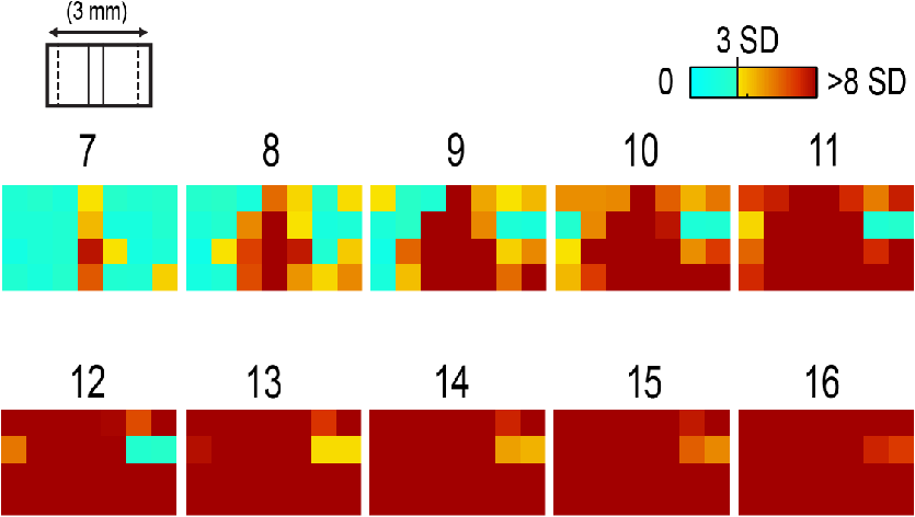

2.5.

Whisker Identity Coding Model Based on Spatial Pattern of Activity

Whisker coding based on mesoscopic patterns of evoked activity was assessed using a two-layer artificial neural network consisting of a $5\times 5$ input layer (“PMBSF” with 25 “whisker barrels”) and a single output unit (downstream “reader” neuron).

The network architecture was similar to a perceptron.²⁴ Input units were only connected to the output unit. There was no feedback onto the input layer. Synaptic weights were randomly set to a value between $-1$ and 1. The degree and arrangement of connectivity between the input and output layers was varied to produce four network types [see Fig. 4(c)]: (1) single connection between input layer and output unit, (2) four adjacent units of input layer connected to output unit, (3) four maximally spaced units of input layer connected to output unit, and (4) all units of input layer connected to output unit. This set of network architectures was chosen because it included variations in the degree of connectivity (1 versus 4 versus 25 inputs) as well as variations in the heterogeneity of connections (adjacent versus spaced inputs).

Each trial consisted of two time steps: (1) activation of input layer and (2) activation of output unit. Input activity was set by empirically derived activity patterns (see below) with values ranging between 0 and 1. Output unit activity was binary (0 or 1) and calculated using a thresholded, linear activation function with no bias constant and threshold = 0.

Input activity patterns were empirically derived from previously published ISOI data.¹⁶ A response decay rate function was derived from average whisker C2-evoked ISOI “initial dip” data obtained by averaging results from 37 rats [Fig. 4(a), left panel]. Four linear sections starting at the peak response and extending radially outward each separated by 90 deg were averaged, peak-normalized, and fitted with a two component exponential function [Fig. 4(a), middle panel]: $0.2\times \exp [-0.07\times (x\times s)]+0.83\times \exp [-0.014\times (x\times s)]$, where $s=21$ to convert from spatial scale of empirical data ($1\text{pixel}=28\mu \mathrm{m}$) to spatial scale of model input layer ($1\text{pixel}=0.5\mathrm{mm}$, approximate distance between barrels in rat PMBSF). The decay rate function was used to produce 25 different activity patterns with peak activation over each of the 25 pixels of the $5\times 5$ input layer [Fig. 4(a), right panel]. Lastly, in order to model changes in stimulus intensity, on every trial the activity pattern was also uniformly scaled by a random factor between 0 and 1 pulled from a uniform distribution function [rand() function in MATLAB^®]. Uniform scaling of mesoscopic response patterns in PMBSF across a wide range of stimulus intensity has previously been shown.¹⁹

Each trial was randomly selected to either include presentation of the target input (C3, with peak activation over the “barrel” at the very center of the $5\times 5$ input layer) or an off-target input (all other whisker inputs). For trials of off-target inputs, one of the 24 nontarget input activity patterns was randomly selected. Thus, half of all trials included the target input, and chance performance had 50% accuracy. Performance (% of trials accurately classified as on or off target) was assessed in blocks of 100 trials called a “session.” Training consisted of 20 sessions (total of 2000 trials) and testing consisted of 10 sessions (total of 1000 trials). Synaptic weights were updated during training (trials 1 to 2000) using the delta rule: $\mathrm{\Delta }{\omega }_{ij}=\alpha \times (t_j-y_j)\times x_i$, where $\omega$ is synaptic weight, $i$ is the presynaptic unit, $j$ is the postsynaptic unit, $\alpha$ is the learning rate constant, $t$ is the target response, $y$ is the actual response, and $x$ is the unit activity. The simulation was repeated for 100 networks (per network type).

Network simulations were repeated for three conditions: (1) no noise, (2) noise, and (3) noise with complex classification task. The no noise condition is described above. For the noise condition, independent noise (random value between $-0.1$ and 0.1) was injected into each unit of the input layer on each trial. For comparison, peak values in input patterns ranged between 0 and 1 with a theoretical mean of 0.5. Thus, the maximum signal-to-noise ratio for peak values under these conditions was 10, with a theoretical average of 5, and even lower signal-to-noise ratios for all off-peak values.

For the last condition, noise was again added and the target input was made more challenging—the output unit had to respond to both the C3 and A5 inputs (while still correctly rejecting all other inputs). MATLAB^® source code at can be found in Ref. 25.

2.6.

Statistics

Cross correlations, modeling, and descriptive statistics were performed using custom MATLAB^® scripts. All parametric statistics were performed in SYSTAT version 11.

For cumulative response magnitudes, responses between 0 and 0.22 mm, 0.5, 1.0, or 1.5 mm from location of peak activity were integrated. For LFP and multiunit (MU) data, response value at 0.22 mm was interpolated (linear interpolation) from response values at 0 and 0.5 mm and the trapezoid method of integration used for cumulative response calculations.

Cross-correlations of evoked LFP with $\pm 50\mathrm{ms}$ lag times were run between pairs of recording locations of an $8\times 4$ array of electrodes using MATLAB’s xcorr() function. Each recording location was used as a seed and cross correlations run with locations within the same vertical column (for vertical connectivity measure) or within the same horizontal row (for horizontal connectivity measure).

For box and whisker plots in Fig. 2, solid line indicates the median, outer bounds of box indicate upper and lower quartiles, whiskers show minimum and maximum values (excluding outliers), and dots represent outliers using the following default formula for box plots in MATLAB^®: maximum whisker length $w$ is set to 1.5 times the interquartile range. Outliers are any data points greater than $q3+w(q3-q1)$ or smaller than $q1-w(q3-q1)$, where $q1$ and $q3$ are the 25th and 75th percentiles, respectively.

Fig. 2

Horizontal and vertical functional connectivity in the barrel cortex. (a) Multielectrode array design to sample from most cortical layers (up to 1.2 mm deep) and across the full breadth of rat barrel cortex (3.5 mm across). (b) Cross correlations on C2 evoked LFP data from Ref. 19 were run for each recording location. Mean $r^2$ values within nearby horizontal recording locations were interpreted as “horizontal” functional connectivity. Mean $r^2$ values for three other electrodes within the bundle were interpreted as “vertical” functional connectivity. (c) Group statistics show stronger functional connectivity along the horizontal axis (within layer) as compared to the vertical axis (within column) for single whisker stimulation (C).

3.1.

Lateral Spread of Whisker Evoked Cortical Activity

The stimulation of a single whisker in rats evokes a prominent lateral spread of activity through PMBSF and into surrounding cortices. An example of a single whisker evoked LFP in PMBSF is shown in Fig. 1, which shows response magnitudes in standard deviations from baseline noise (see Sec. 2 for details). Every sampling location—which included electrodes from four different cortical layers extending beyond the boundaries of PMBSF—recorded evoked LFP that was over three standard deviations above baseline noise. These data suggest that evoked activity is only constrained to a cortical column for 1 ms following single whisker stimulation, before spreading laterally beyond columnar boundaries and engaging a broad volume of cortex.

Robust horizontal functional connectivity would be consistent with the prominent lateral spread of evoked activity; however, this has not been explicitly tested before. Therefore, functional connectivity along vertical and horizontal domains in PMBSF was compared using cross-correlations of multisite recordings of a single whisker (C2) evoked LFP (Fig. 2). Correlation coefficients for cross-correlations with a seed location were binned vertically or horizontally [see representative seed map in Fig. 2(b)] and then averaged for all seed locations. Mean peak $r^2$ values were significantly higher for horizontal connectivity compared to vertical connectivity [$p=0.001$ paired $t$-test; Fig. 2(c)]. These data suggest a robust horizontal connectivity that is stronger than the well-established vertical connectivity in PMBSF.

3.2.

Prominent Cumulative Evoked Activity Beyond Columnar Boundaries

Stimulation of a single whisker in rats evokes responses within columns of cortical tissue in PMBSF that rapidly spreads laterally into surrounding cortices (Fig. 1). The cortical response to single whisker stimulation can thus be broken into two components: peak responses localized within cortical columns (strong response, small volume, Fig. 3, blue responses) and a broad profile of weaker responses (weak response, large volume, Fig. 3, orange responses). To determine whether most single whisker evoked activity in PMBSF occurs near peak responses (i.e., within columnar boundaries) or in surrounding cortices (i.e., beyond columnar boundaries), cumulative response magnitudes were calculated.

Fig. 3

Single whisker evokes more activity outside the barrel column. (a) Schematic of single whisker and anatomical representation in PMBSF. (b, e, h) Single whisker evoked activity in PMBSF measured by ISOI “initial dip” signal (b, data set from Ref. 16), LFP (e, data set from Ref. 19), and multiunit activity (h, data set from Ref. 19). FC, fractional change. (c, f, i) Mean response magnitudes at 0, 0.5, 1, and 1.5 mm from location of peak c2 evoked response for (c) ISOI, (f) LFP, and (i) MU activity. (d, g, j) Cumulative responses at 0.22, 0.5, 1.0, and 1.5 mm from location of peak C2 evoked response for (d) ISOI, (g) LFP, and (j) MU activity. (d) For two-dimensional ISOI data, responses were integrated within specified radius. (g, j) For one-dimensional electrophysiology data, responses were integrated between 0 mm and specified distance from peak response. Responses at 0.22 mm were estimated using linear interpolation. (e, h) Representative single whisker evoked LFP (e) and multiunit PSTHs (h) at increasing distances from peak response. $\text{Recording depth}=600\mu \mathrm{m}$. Solid black line in b denotes PMBSF boundary.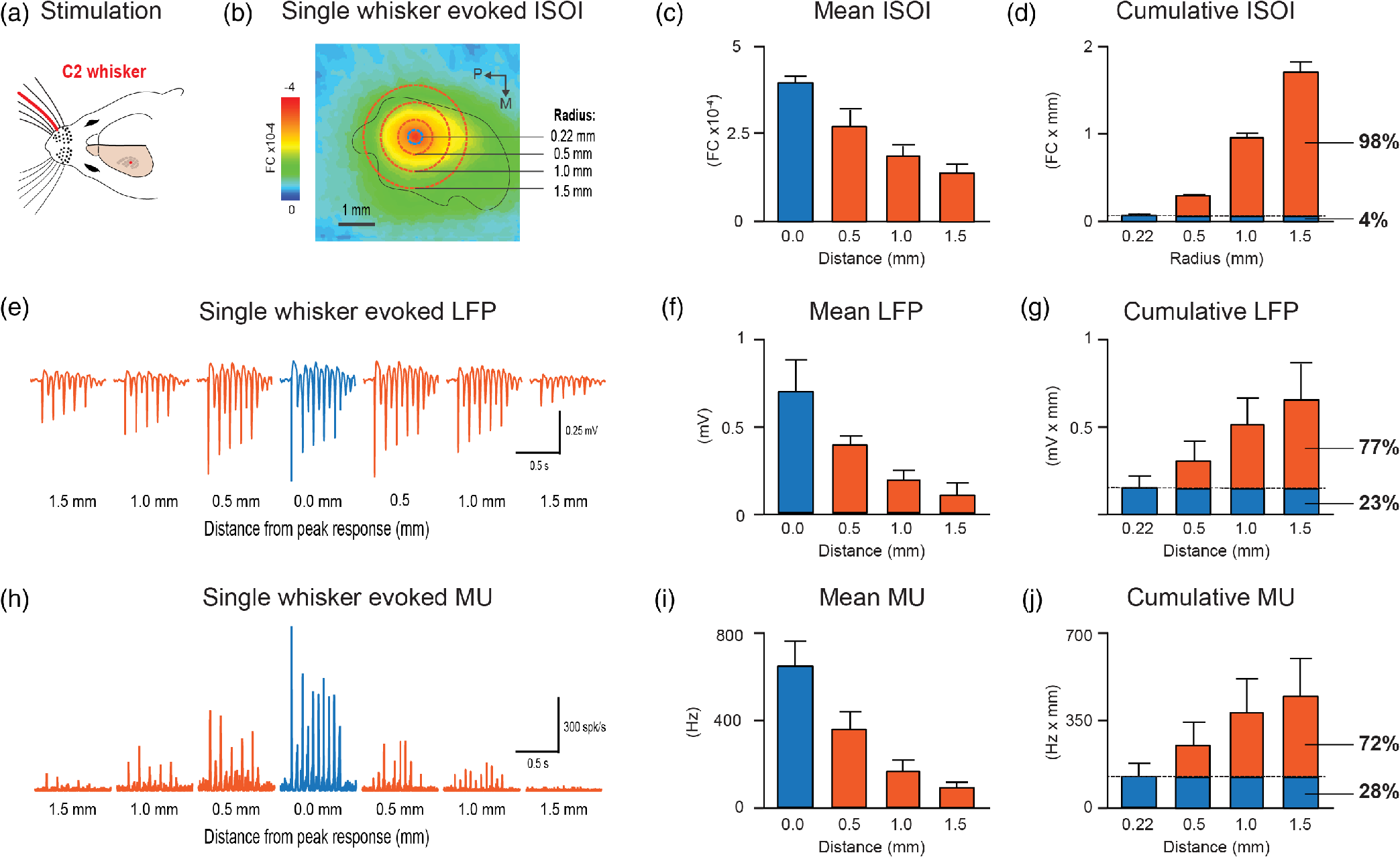

Following single whisker C2 stimulation [Fig. 3(a)], cumulative response magnitudes (response magnitude integrated across space) were calculated for increasing distances/areas from the location of peak responses for ISOI initial dip data [Fig. 3(d), $n=37$, data set from Ref. 16], LFP [Fig. 3(g), $n=6$, data set from Ref. 19], and multiunit activity [MU, Fig. 3(j), $n=6$, data set from Ref. 19]. A distance/radius of 0.22 mm was used as the standard demarcation for columnar boundaries based on the $0.15{\mathrm{mm}}^2$ area of the C2 whisker barrel.⁹ Cumulative response magnitudes were calculated up to a distance/radius of 1.5 mm, roughly corresponding to the boundaries of PMBSF as measured from the C2 whisker barrel. On average, the cumulative response between 0 and 0.22 mm from peak responses (i.e., total activity within columnar boundaries) was only 4%, 23%, and 28% of the cumulative response between 0 and 1.5 mm from peak responses (i.e., total activity within and beyond columnar boundaries, up to 1.5 mm) for ISOI, LFP, and multiunit data sets, respectively. The lateral spread of evoked multiunit activity tends to be more spatially restricted than evoked LFP¹⁴ and ISOI activity,¹⁶ which could explain the range in cumulative response magnitudes beyond columnar boundaries. For both activity measures, these data show that the vast majority of whisker-evoked activity (as much as 98%, for ISOI data) occurs beyond columnar boundaries. These percentages would be even smaller if the entire lateral spread of evoked activity, which extends beyond PMBSF boundaries,¹⁴ were included.

3.3.

Robust Whisker Identity Coding Using Evoked Activity Spread

What is the purpose of all this extracolumnar activity? A possible role in providing a robust foundation for whisker coding is explored.

Robust coding of whisker identity with spatial activity patterns was tested using a two-layer artificial neural network model of PMBSF and a downstream “reader” neuron. The input layer of the network was a $5\times 5$ grid representing a simplified model of PMBSF with 25 whisker barrels separated by 0.5 mm [Fig. 4(a), right panel]. The pattern of activity across the input layer was empirically derived from C2-evoked ISOI “initial dip” data,¹⁶ which was used to create a standard curve for the decay rate of single whisker evoked point spreads in rat PMBSF [Fig. 4(a), middle panel]. The simplified $5\times 5$ patterns of activity were used to demonstrate an inherent ambiguity in whisker evoked columnar activity and, combined with downstream “reader” output units, to test whether spatial patterns of activity could support a robust whisker identity coding mechanism.

Fig. 4.

Spatial patterns of activity support robust whisker identity coding scheme. A simple two-layer neural network model was used to test the robustness of whisker coding based on large spatial patterns of cortical activity. (a) Simplified cortical activity patterns were derived from mean whisker C2-evoked ISOI “initial dip” data from rat PMBSF ($n=37$, data set from Ref. 16). Left panel, mean ISOI “initial dip” data used to fit the decay rate function. Middle panel, ISOI response magnitudes plotted against cortical distance from peak response (black circles) with overlay of fitted response decay function (blue line). Right panel, example of a $5\times 5$ stimulus pattern ($1\text{pixel}=0.5\mathrm{mm}$) generated by the response decay function. Scale bar, $\text{left panel}=1\mathrm{mm}$. (b) Before being used as inputs into the model, stimuli were multiplied by a randomized scalar to capture the variable intensity of whisker stimuli (left panel). Each whisker stimulus would therefore vary greatly in absolute response magnitude from trial to trial while the relative pattern of activity remained exactly the same, consistent with a previous report of invariant relative spatiotemporal profile of activity across large ranges of stimulus intensities.¹⁹ Given the slow response decay rate, these conditions made it effectively impossible to classify whisker stimulus identity (e.g., whisker C3) using responses at any one location (middle panel). If responses from two locations are considered, the classification problem is greatly simplified (right panel). (c) Gray, reader unit connected to single location of input layer located at the peak response for the target stimulus (C3). Red, reader unit connected to four adjacent units of the input layer all within close proximity to the peak response for target stimulus. Blue, reader unit connected to four units of the input layer, one at the location of peak response for target stimulus and three additional units at maximal distances from the first. Green, reader unit connected to all units of the input layer. (d) Whisker classification performance for each reader type. Classification accuracy for all readers was tested in three conditions of increasing difficulty: no noise (left panel), noise (middle panel), and noise with a complex target where readers had to respond to both the C3 whisker pattern as well as the A5 whisker pattern (right panel, “complex target”). $\text{Error bars}=\mathrm{SEM}$.

If input patterns are scaled by a random factor across trials [Fig. 4(b), left panel], there is no simple way of classifying whisker identity using input activity from just one location of the input layer [Fig. 4(b), middle panel]. This would be analogous to receiving afferents from neurons in a single cortical column. The difficulty in classifying whisker stimulus identity using activity from a single cortical location arises from the overlap in response magnitude distributions produced by a range of possible whisker stimulus intensities. For example, weak stimulation of the C2 whisker may produce a weaker response in the C2 barrel than strong stimulation of the C3 whisker. A simple way to resolve this inherent ambiguity is to integrate activity from multiple locations across PMBSF [Fig. 4(b), right panel].

Four network architectures with varying degrees of connectivity between the input layer and the output unit were investigated [Fig. 4(c)]. Classification performance of each network architecture was compared across three conditions of increasing difficulty—no noise [Fig. 4(d), left panel], noise [Fig. 4(d), bottom middle panel], and noise with a complex target [Fig. 4(d), right panel]. Results show that performance above chance (50%) required readers to be connected to multiple units of the input layer [Fig. 4(d), compare gray circles to all other circles]. Performance improved if the reader was connected to more heterogeneous units of the input layer [Fig. 4(d), compare blue and red circles]. Performance was best if the reader was fully connected to the entire input layer [Fig. 4(d), compare green and blue circles]. These results show that using the full spatial profile of activity [Fig. 4(d), green network and circles] can support whisker coding that is robust to random scaling of input patterns, local noise designed to produce an average signal-to-noise ratio of 5 for peak responses and 2.5 for more distal responses ($+1.5\mathrm{mm}$ from peak response, see Sec. 2 for details), and supports learning a classification scheme in which the output unit responds to either of two nonadjacent whiskers but not to any others [with 85% accuracy for fully connected output unit, Fig. 4(d), right panel, green circles].

In summary, these results suggest that stimulating a single whisker engages the entirety of PMBSF (Fig. 1) with stronger horizontal functional connectivity than vertical functional connectivity (Fig. 2), evokes more activity beyond columnar boundaries than within (Fig. 3), and produces spatial patterns of activity that support highly robust whisker identity coding (Fig. 4).