Improving voltage-sensitive dye imaging: with a little help from computational approaches

Sandrine Chemla; Lyle Muller; Alexandre Reynaud; Sylvain Takerkart; Alain Destexhe; Frédéric Chavane

doi:10.1117/1.NPh.4.3.031215

19 May 2017 Improving voltage-sensitive dye imaging: with a little help from computational approaches

Sandrine Chemla, Lyle Muller, Alexandre Reynaud, Sylvain Takerkart, Alain Destexhe, Frédéric Chavane

Author Affiliations +

Neurophotonics, Vol. 4, Issue 3, 031215 (May 2017). https://doi.org/10.1117/1.NPh.4.3.031215

Abstract

Voltage-sensitive dye imaging (VSDI) is a key neurophysiological recording tool because it reaches brain scales that remain inaccessible to other techniques. The development of this technique from in vitro to the behaving nonhuman primate has only been made possible thanks to the long-lasting, visionary work of Amiram Grinvald. This work has opened new scientific perspectives to the great benefit to the neuroscience community. However, this unprecedented technique remains largely under-utilized, and many future possibilities await for VSDI to reveal new functional operations. One reason why this tool has not been used extensively is the inherent complexity of the signal. For instance, the signal reflects mainly the subthreshold neuronal population response and is not linked to spiking activity in a straightforward manner. Second, VSDI gives access to intracortical recurrent dynamics that are intrinsically complex and therefore nontrivial to process. Computational approaches are thus necessary to promote our understanding and optimal use of this powerful technique. Here, we review such approaches, from computational models to dissect the mechanisms and origin of the recorded signal, to advanced signal processing methods to unravel new neuronal interactions at mesoscopic scale. Only a stronger development of interdisciplinary approaches can bridge micro- to macroscales.

1. Introduction

Despite the tremendous recent advancements in neuronal activity recording tools, voltage-sensitive dye imaging (VSDI) remains the only technique that allows to measure neuronal activity with high temporal (1 to 10 ms) and spatial ( $< 50 μ m$ ) resolution¹^,² over a large field-of-view (typically about 1 to $2 {cm}^{2}$ ). VSDI² thus provides access to the mesoscopic scale, i.e., a network of neurons from the column to a whole area, between microscopic (single-neuron) and macroscopic (whole-brain) scales. Recording techniques providing access to this scale—VSDI as well as by other optical imaging techniques (e.g., optical imaging of intrinsic signals, two-photon microscopy) and multielectrode arrays [Fig. 1(a)]—have unfortunately received relatively little attention from the neuroscientific community: only 4% of publications listed in PubMed with the keyword “cortex” study this mesoscopic scale, with only 0.5% from VSDI [Fig. 1(b) and Table 1]. This relative lack of attention stands in contrast to the fact that more than 95% of interneuronal connections occur between neurons separated by less than 2 mm in cortex.⁴ These under-explored techniques, with VSDI in particular because it remains unique in the field-of-view and temporal resolution it reaches, have, therefore, an enormous potential for unraveling new fundamental scientific discoveries. Two points, however, stand in the way of this potential: (1) insufficient understanding of the VSDI signal’s origin and (2) the lack of standardized signal processing tools. Developing dedicated computational approaches may, therefore, be the key to improve our knowledge and know how in VSDI studies.

Fig. 1

Spatio-temporal resolution and scales of neuronal recording methods. (a) Three-dimensional representation of 10 families of neuronal recording methods as a function of their spatial resolution, temporal resolution, and the spatial field-of-view that they can reach.² INTRA, intracellular recordings; S/MUA, single or multiunit activity; LFP, local-field potentials; 2-PH, two-photon microscopy; MEA: multielectrode array; VSDI, voltage-sensitive dye imaging; OI-IS, optical imaging of intrinsic signals; fMRI, functional magnetic resonance imaging; E/MEG, electro- or magneto-encephalogram; IDEAL, the ideal technique. (b) In the same spatial resolution, field-of-view representation, frequency histograms of the amount of publication referenced in PubMed with the word “cortex” and one of these method. The generic search line was: (TECHNIQUE_NAME[Title/Abstract]) AND (cortex[Title/Abstract] OR cortical[Title/Abstract]). When appropriate, the technique name was written in full and abbreviated.

Here, we review recent advances in that direction. First, we describe how generative models of VSDI data can help to better understand the origin of the signal and unravel possible underlying mechanisms. In particular, biophysical models have proved very useful in describing the signal’s multicomponent origin. Second, we strongly suggest a standardization of signal processing tools that are key for generalization and comparison of results obtained with VSDI. With this imaging technique, the raw signal is corrupted by many noise components arising from physiological, mechanical, or electronical sources. We review the signal processing tools that have been developed for VSDI signal analysis. Finally, we show that combining single-trial data analysis with computational models can reveal the origin of the observed signal’s dynamics. Similar to the convergent interdisciplinary efforts that have been undertaken to optimize our understanding and use macroscopic brain imaging signals [i.e., functional magnetic resonance imaging (fMRI), magneto-encephalogram, and electro-encephalogram], we believe that such computational approaches are needed for the development of VSDI and are vital to establishing this as a standard neuroscientific imaging technique.

Table 1

Orders of magnitude of neuronal recording techniques in terms of spatial resolution, temporal resolution, and field-of-view,2,3 as well as the exact hit in PubMed search.

	INTRA	S/MUA	LFP	2-PH	MEA	VSDI	OI-IS	fMRI/TEP	E/MEG	IDEAL
Spatial resolution	Subneuronal	Neuron	Neuron-column	subneuronal	Neuron	Neuron-column	Neuron-column	Subareal	Subareal	Subneuronal
Field-of-view	Neuron	Neuron	Column	Column	Multicolumns	Area	Area	Brain	Brain	Brain
Temporal resolution	Sub-ms	ms	Tens of ms	Tens of ms	ms	ms	Hundreds of ms	Hundreds of ms	Hundreds of ms	Sub-ms
Pubmed search:	10,267	8680	739	784	572	346	964	24,943	16,131

2. Computational Models of Voltage-Sensitive Dye Imaging Signal

We start by reviewing the different computational models available to better understand the origin of the population dynamics and the VSDI signal.

2.1.

Dissecting the Underlying Mechanisms of the Response Dynamics

The behavior of large assemblies of neurons can be studied without having to tackle the mathematically unwieldy challenges associated with microscopic considerations. Indeed, at the mesoscopic scale, it is valid to study average values, thus requiring only simple computations to describe the activity of interacting populations of neurons through mean-field theory.⁵ The VSDI signal reports mesoscopic population activity at high spatio-temporal resolution and has been successfully reproduced by models developed at this scale.⁶^–¹⁵ Here, we briefly review, in a nonexhaustive manner, three families of such models (see Ref. 14 for a more detailed overview of the models and their equations).

2.1.1.

Neural-field models

Grimbert and Chavane,¹⁰ as well as Markounikau et al.¹³ and Deco and Roland,¹⁴ proposed neural fields as a suitable mesoscopic model of cortical areas. Neural fields are continuous networks of interacting neural masses, describing the dynamics of the cortical tissue at the population level.¹⁶ Therefore, they are appropriate to solve the direct problem of the VSDI signal, i.e., to generate a VSD signal given the neural substrate parameters and activities. These three models indeed account for physiological spatio-temporal dynamics of V1 population responses to various illusory motion stimuli (apparent motion, line motion).

2.1.2.

Self-organizing models

The laterally interconnected synergistically self-organizing map (LISSOM) family of models¹⁷^,¹⁸ was also proposed to reproduce the spatial organization of V1 as observed with optical imaging. It is based on Hebbian self-organizing algorithms¹⁹ used to visualize and interpret large, high-dimensional data sets. Sit and Miikkulainen⁹ but also Stevens et al.⁶ proposed variants of the original LISSOM model to account for the development of stable and realistic cortical functional maps.

2.1.3.

Conductance-based models

Rangan et al.⁸ proposed a large-scale conductance-based integrate-and-fire (IAF) model of the primary visual cortex in order to reproduce the spatiotemporal activity patterns of V1, as revealed by VSDI, in response to the line motion illusion.²⁰ This family of models simplifies the model of Hodgkin and Huxley (HH) by representing neurons as IAF units while still taking into account a simplified version of the conductance changes due to action potentials.²¹ More recently, Chizhov¹⁵ also used this family of models to account for VSDI dynamics.

Each of these models helps understanding or testing the role of some specific components of the VSDI signal. For instance, one intriguing feature of VSDI cortical responses to illusory motion stimuli,²⁰^,²² calls for the existence of slow mechanisms that can “bind” spatially and temporally the transient stationary inputs composing the stimulus sequence. In all models, such nonlinear low-pass filtering by the neuronal population has been attributed to various mechanisms. For instance, Markounikau et al.¹³ and Chemla and Chavane²³ both suggested that a balance between excitation and inhibition and lateral connections are potential mechanisms shaping the sequence of stationary input. Similarly, Chizhov¹⁵ found that intracortical connectivity is a critical factor accounting for VSDI dynamics. In Ref. 8, the NMDA conductance has been further proposed as a complementary, nonexclusive, mechanism to account for the slow dynamics of the VSDI signals. Such a conductance could also play an important role in structuring on-going spontaneous activity by generating an intermittent unsuppressed state.²⁴ These results show that computational models can be used to demonstrate the plausibility of various mechanisms probed by specifically incorporating the putative candidate, conductances, or connectivity—such as horizontal and vertical intercolumnar connections between neural masses¹⁰ or feedback.¹⁴ However, none was specifically designed to dissect the origin of the VSDI signal, which is a central question for interpreting the results (see Ref. 14 for a detailed review on this problematic). The VSDI technique is indeed a complicated signal based on voltage-sensitive dyes that bind to the cells’ membrane and linearly transform variations in the membrane potential into fluorescence. A millisecond temporal resolution is reached by using a highly sensitive charge-coupled device camera, whereas the spatial resolution (down to 20 to $50 μ m$ ) is mainly limited by optical scattering of the emitted fluorescence.²⁵ The recorded signal, therefore, results from fluorescence integrated over a large population of cells and is thus affected by activity of intermingled components under each measuring pixel, e.g., different neuronal compartments (including dendrites, somata, and axons) of different cell types (excitatory and inhibitory) in different layers, which are likely to be stained in the same manner. How to isolate the contributions from its different components is, therefore, a difficult question to answer directly. To specifically investigate this question, Chemla and Chavane²³ have proposed a biophysical model that we present below.

2.2.

Biophysical Model for Unraveling the Signal’s Origin

2.2.1.

Basics of the model

We developed a detailed biophysical cortical column model based on known neural properties of the visual cortical network and adjusted to reproduce the dynamics of experimental VSDI signal.²⁶^,²⁷ The model was developed at a scale that corresponds in size to one pixel of the VSDI image ( $50 μ m$ ) and embedded into a larger network to be realistic, i.e., an artificial hypercolumn (in the case of V1). More precisely, this model comprised 180 multicompartment HH neurons [see Fig. 2(a)] with three different types of excitatory neurons (one type per represented layer) and one unique type of inhibitory neurons in each of the three layers (2/3, 5, 5/6). Excitatory and inhibitory neurons, which represent 80% and 20% of the cells respectively, were initially fitted to intracellular recordings from Ref. 28. These neurons were then recurrently connected in accordance with Ref. 29, which provided a quantitative estimation of the synaptic projections between these different neuronal types. The local network calibration was done by tuning the contrast response functions of these two populations of neurons to reproduce those obtained electrophysiologically in vivo.³⁰ Lateral interactions were tuned in strength and number of synapses to fit excitatory and inhibitory distributions, respectively, from Refs. 31 and 32. Background activity was also taken into account in the form of fluctuating ionic conductances³³ in order to reproduce in vivo synaptic bombardment. Finally, the dye attenuation parameter was given by the distribution of fluorescence intensity estimated by Ref. 34.

Fig. 2

VSDI biophysical model schematic and contributions. (a) Model representation. The six populations of neurons, depicted by one unique representative neuron (small pyramidal cells in layer 2, spiny stellate cells in layer 4, large pyramidals in layer 5, and smooth stellate cells in each layer), are recurrently connected (red arrows). The cortical column is embedded into a larger network by simulating a realistic synaptic bombardment on each population (green arrows) and by modeling lateral connections between the column and its neighbors (blue dashed arrows). Inputs from the thalamus to layer 4 neurons are represented by the large red arrow on the left. (b) Time-course of the modeled VSDI signal (red trace) in response to a thalamic input of 800 ms (black trace), compared to the experimental signal (gray trace) obtained in monkey V1. (c) Correlation analysis between the VSDI signal and the membrane potential of each compartment of the column for three periods of time (spontaneous activity, stimulation onset, or rising phase and evoked activity). (Adapted with permission from Ref. 23. Copyright © 2010.)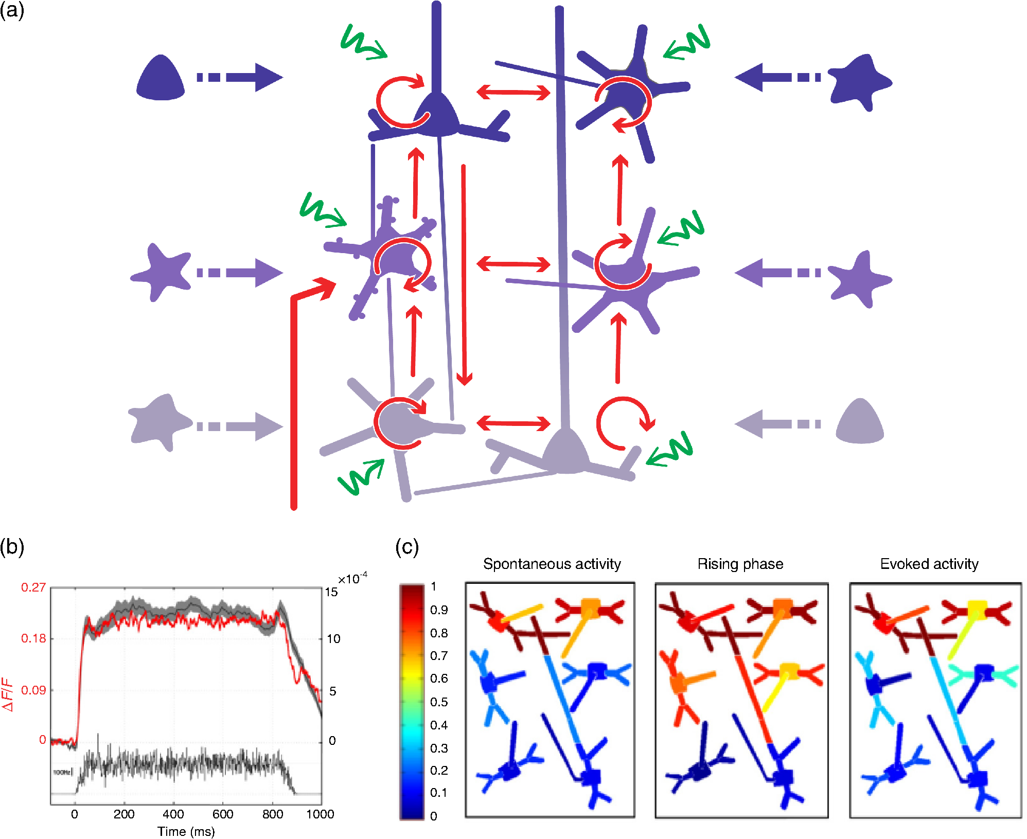

2.2.2.

Unraveling time and stimulus-dependent origin of the signal

We computed the VSDI signal by linearly integrating the membrane potential over the total surface area, corrected by a factor accounting for the amount of staining of each compartment. This model reproduced well the experimental VSD signal dynamics [Fig. 2(b), in black the $mean \pm SEM$ of the recorded VSDI and in red the modeled VSDI]. At this stage, the model was used to quantify the different contributions of the signal, by computing the fraction of the contribution of each compartments, but also the correlation between each of these compartment and the global signal [represented graphically in Fig. 2(c)]. Importantly, the model was very stable and tolerant to changes in the model’s parameters (synaptic weights and number of connections).

As expected, the VSDI signal mainly reflects dendritic activity of excitatory neurons in superficial layers [gross contribution of 60%, high level of correlation in Fig. 2(c)], with 40% of the signal originating from a mixed contribution of inhibitory neurons, lower layers, and axons (hence spikes). However, when increasing the thalamic input strength, these contributions are changing, inhibitory cells contribution increase, and the one of axons decreases. Importantly, these contributions are also dynamic: the contribution and level of correlation from layer 4 neurons and inhibitory neurons, as well as axons, increased transiently at response onset [Fig. 2(c)].²³ This model hence demonstrated that the relative contribution of all compartments is not stationary and that no compartment on his own allows to fully account for the global signal.

2.2.3.

Effect of anesthesia and the notch as a marker of transient imbalance of excitation/inhibition

In a recent extension of this model, we further probed how much these contributions will depend on the network state since studies in VSDI are both done in anesthetized and awake preparations.³⁵ Succinctly, we manipulated a key model parameter to account for the effect of anesthesia: the decay time constant tauG of GABA_A-mediated IPSCs. Indeed, tauG has been shown to be prolonged in a dose-dependent manner by most anesthetics as reported in Ref. 27. Figure 3(a) shows that, when increasing tauG, our model predicted that the VSDI signal amplitude should decrease and the transient imbalance between excitation and inhibition increase. These predictions were confirmed experimentally with monkeys at different arousal states, induced by the administration of midazolam, i.e., a positive GABA_A modulator, during a behaving session [Fig. 3(b)]. Altogether, these results provide a quantitative description of the effect of GABA_A receptor modulation on the cortical population dynamics, as measured by the VSDI signal. Interestingly, our model predicted that one key feature of the VSDI signal, the so-called “deceleration–acceleration (DA) notch” component introduced by Sharon and Grinvald³⁶ as “a small transient drop in the rate in which the evoked response increased,” is resulting from desynchronization between excitation and inhibition induced by anesthesia. Physiological recordings in awake and anesthetized preparation confirmed this prediction. The DA notch was indeed proposed to be an emergent signature of the cortical network excitability.³⁶^–³⁸ Chemla and Chavane’s study further demonstrated that this is a prominent property of VSDI in anesthetized state and could be taken as a marker of a transient imbalance between excitation and inhibition. This effect is logical since anesthetic specifically slows down inhibitory conductances and not excitatory. At response onset, inhibition will have the possibility to transiently override excitation, before being re-equilibrated by the strongly recurrent cortical network.

Fig. 3

Model predictions on the effect of anesthesia and experimental validation. (a) Effects of tauG modulation on the modeled VSDI signal dynamics (Plateau and DA notch amplitude). Top row: onset of the normalized VSDI signal time-courses decomposed into excitatory (burgundy traces) and inhibitory (orange traces) cells activity for three tauG values (2.5, 5, and 10 ms), revealing the DA notch formation. Middle row: time-course of the difference between excitatory and inhibitory VSDI signals. Bottom row: boxplot diagrams of the plateau amplitude (left) and the DA notch amplitude (right) of the modeled VSD response as a function of tauG. Significant differences with the condition $tauG = 2 ms$ ( $P < 0.01$ ) are denoted by a star. (b) Experimental validation of the model predictions shown in (a). Top row: onset of the experimental VSDI signal time-courses obtained in three awake (left) and three anesthetized (right) monkeys, in response to full-field drifting gratings of high contrasts. One monkey was recorded in both arousal conditions (dashed lines). Bottom row: Boxplot diagrams of the Rmax or plateau amplitude (left) and DA notch amplitude (right) values of the experimental VSDI data shown on top. (Adapted with permission from Ref. 35. Copyright © 2016.)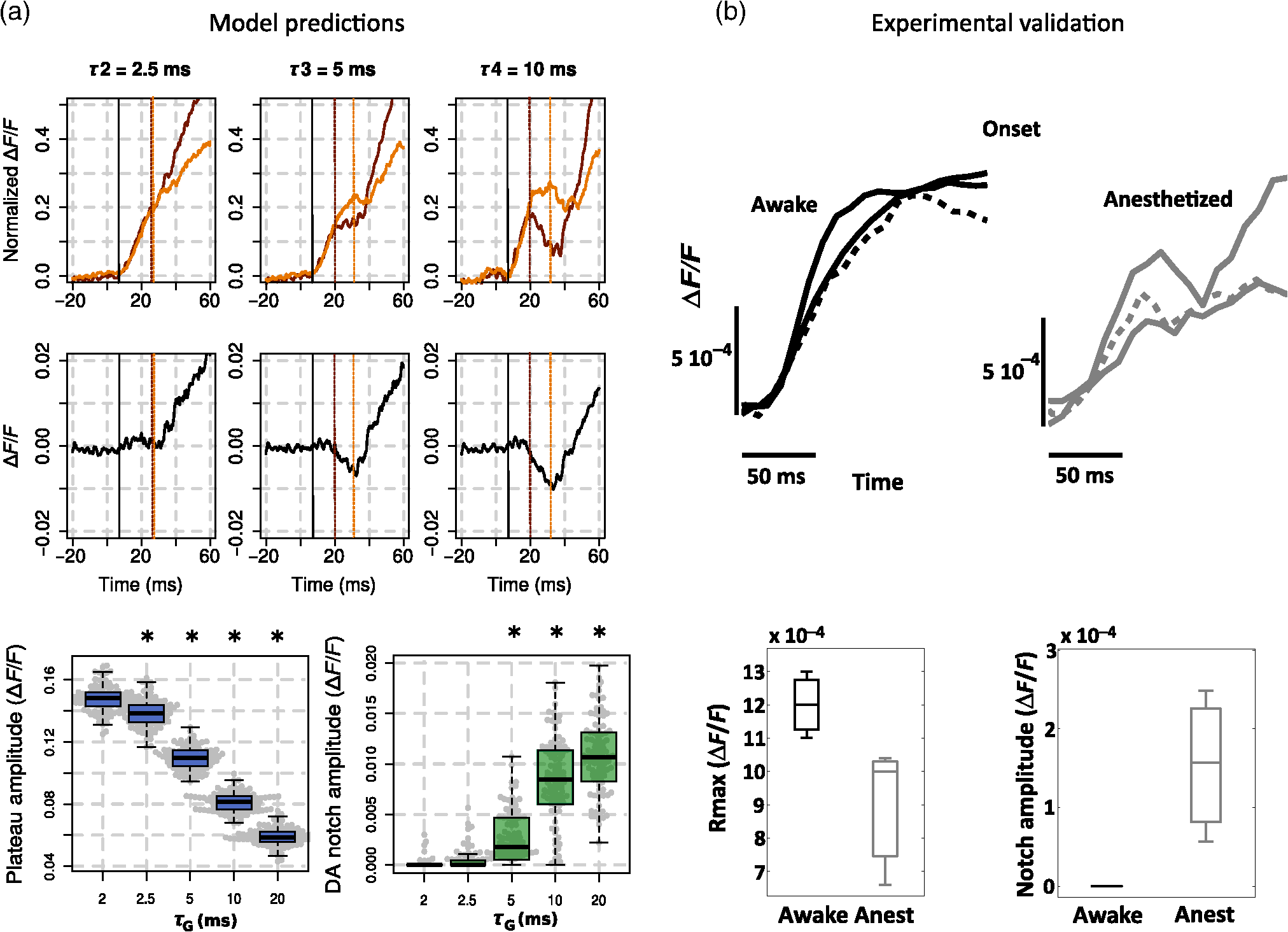

VSDI generates complex experimental data that are difficult to interpret. Computational models can help explain the origin of this signal. These models are useful to understand the role of the major components of the VSDI signal and to generate experimentally testable predictions. However, the validation of such models cannot be achieved in isolation to real experiments, which are necessary to constrain them. In order to facilitate the confrontation of computational models and real data, it is, therefore, necessary to improve the signal processing algorithms available for VSDI data, and we now review the recent literature dedicated to this.

3. Signal Processing Methods for Improving Voltage-Sensitive Dye Imaging Signals

3.1.

Review of the Different Methods

The raw VSDI signal is a noisy combination of several different components. We describe below the three main families of denoising methods that have been proposed to extract the neuronal signature from VSDI data.

3.1.1.

Blank subtraction

The most common and first empirical denoising method is the blank subtraction.¹^,³⁹ It consists in estimating noise components using blank trial recordings (no stimulation) or a “cocktail blank” consisting of the mixture of all other stimulation conditions.⁴⁰ The first step of the analysis consists of dividing each image of the stack by the first frames (recorded before stimulus onset) in order to correct for inhomogeneous levels of illumination and staining. In the second step, image stacks collected during stimulated trials are subtracted by those acquired during blank trials on a frame-by-frame basis. This subtraction aims at removing the slow drifts due to dye bleaching as well as synchronous physiological artefacts like heartbeat.¹ A decaying general trend often persists, however, which can be attributed to change in bleaching dynamics or physiological parameters. Therefore, a subsequent linear detrending step can be applied.⁴¹^,⁴² Some more statistically reliable measure can then be applied, such as a $z$ -score taking into account the level of variability pixel by pixel.²⁰^,⁴³

However, this blank subtraction method presents several limitations. The most important is that the first frames division is an inaccurate normalization method⁴⁴ and leads to a systematic misestimation of the intertrial variance dynamics.

3.1.2.

Blind sources separation techniques

The first decomposition technique applied in intrinsic optical imaging was principal components analysis.⁴⁵^,⁴⁶ The signal is decomposed using an automatic algorithm but signal versus noise modes need to be identified a posteriori, often using ad hoc statistical criteria. This was later improved by using multitaper harmonic analysis.⁴⁷ However, noise sources synchronized on acquisition or stimulus onset can remain embedded in selected modes. Further improvements have been proposed, such as extended spatial decorrelation,⁴⁸^,⁴⁹ which uses spatial statistical features to separate the recorded mixed sources, or indicator functions,⁵⁰^–⁵² which are determined upon stimulated/reference trials comparison.

The second main decomposition processing family is independent components analysis (ICA),⁵³ which relies on the extraction of the original sources by maximizing their statistical independence. ICA has been mostly applied on VSDI recordings in anesthetized preparations at the single-trial level. A posteriori component identification also mostly relies on statistical criteria⁵⁴^,⁵⁵ or with a “weak model” on intrinsic optical imaging data.⁵⁶ Again, these decomposition techniques focus on the temporal dimension and can easily be combined with complementary spatial routines such as spatial ICA⁵⁷ or local similarity minimization.⁵⁸ As noted above, the modes are not determined upon physiological criteria but upon signal statistics. Thus, nothing guarantees perfect source separation and parameters estimation is impossible.⁵⁹ Signal and noise modes can also be classified as user judgment after decomposition, for instance based on complementary recordings.⁶⁰

These techniques can also be successfully applied on datasets obtained with specifically designed paradigms with periodic stimuli. There, the effective separation of the stimulus-evoked responses from noise is done with Fourier analysis, first developed for fMRI mapping⁶¹ and then applied to intrinsic⁶² and voltage-sensitive dye imaging.³⁸^,⁵⁹^,⁶³

3.1.3.

Linear regression techniques

A different solution lies in multiple linear regression techniques, which were initially developed for fMRI⁶⁴ and were subsequently adapted to various optical imaging techniques: intrinsic imaging,⁵⁶^,⁶⁵^,⁶⁶ blood flow,⁶⁷ calcium fluorescence,⁶⁸ synaptoPhluorin fluorescence,⁶⁶ and VSDI.⁶⁹ These techniques are based on explicit decomposition of all signal components, mostly by identification of their physical sources. These components are then used to build a regression matrix on which the signal will be projected. The shape of the regressors, therefore, has to be modeled a priori. By construction, this technique has several advantages—it is applied at single-trial level, can specifically identify nonreproducible artefacts, and discounts for any bias in component selection. As with the other techniques, it can also be further constrained by the spatial structure of the signal.⁷⁰

3.2.

GLM for Recovering Single Trials

One key issue in linear regression techniques is the definition of components. They can be defined as templates or mathematical models. Templates can be used to model components that are very reproducible across trials and do not present any other changes than gain amplitude. Several studies have successfully used templates for modeling response components in intrinsic, synaptophluorine,⁶⁶ or calcium imaging.⁶⁸ However, they do not allow to account for changes in latency, duration, or shape, as seen in VSDI. One solution is to manually decompose the expected response in several template components,⁶⁵^,⁶⁷ but this is only possible when changes in response shape are small, as in intrinsic imaging.

To overcome these technical limitations, important improvements come from the use of fMRI’s linear optimal basis sets (FLOBS) initially designed for fMRI⁷¹^,⁷² in order to extract the activity dynamics in the VSDI signal and to model several evoked response shapes.⁶⁹^,⁷⁰^,⁷³ A set of temporal regressors is determined by a singular value decomposition of a large set of simulated possible changes in the response. Then, few first eigenvectors are kept and included as regressors in the model. Such model is then able to selectively extract, independently for each pixel and each trial, a large range of temporal dynamics of responses evoked by different sets of stimuli, including changes in amplitude, duration, and delay. It should be noted, though, that in linear regression, good source separation requires that all the vectors of the new basis are orthogonal. Thus, when building the regression matrix, one must check that the nonneural components are orthogonal to the stimulus-evoked response ones in order to ensure that the evoked response signal is not embedded in noise regressors and that sensory-driven response estimated by the model is not corrupted by the noise sources. This is usually trivial for VSDI data as noise components often show a much faster dynamic and periodicity than response ones.

Figure 4(a) shows the model design used by Reynaud et al.⁶⁹ to denoise VSDI data acquired in the awake monkey. The noise and response components are modeled in the following steps. The first noise component represents the baseline level $X_{0}$ by a constant value. Electronic⁷⁴ and physiological artifacts $X_{1}$ (Ref. 1) are characterized by periodic oscillations and are thus modeled with Fourier series, allowing for phase changes. Finally, the dye bleaching can be defined with exponential functions $X_{2}$ .⁷⁵ The response components $X_{3}$ are the FLOBS and describe the neuronal response. The decomposition of the temporal signal on the basis of all these regressors will lead to the identification of individual coefficients. Finally, the response components and the residual can be extracted and normalized by $X_{0}$ to reconstruct the denoised response [Fig. 4(b)].

Fig. 4

Linear model decomposition. (a) A raw trial is linearly decomposed into noise components ( $X_{0}$ baseline, $X_{1}$ periodic components, and $X_{2}$ bleaching components), the evoked response components ( $X_{3}$ ), and the residual. $F$ denotes fluorescence. (b) Linear model denoising scheme. The reconstructed signal is the sum of the response components ( $X_{3}$ ) and the residual, divided by the baseline illumination level to obtain a normalized reconstructed signal ( $Δ F / F$ ). (c) Example of the linear model application on two trials in response to a-600 ms visual stimulation in the monkey visual cortex. First column: raw trials (black) and bleaching component (as estimated with the linear model; gray). Second column: other components estimated with the LM: evoked response (red) and periodic noise components (gray). Third column: residuals. Last column: estimated responses using the linear model denoising scheme (LM; red) and the standard blank subtraction (BkS; blue). Note the different scales on the ordinates axis. Adapted with permission from Ref. 69.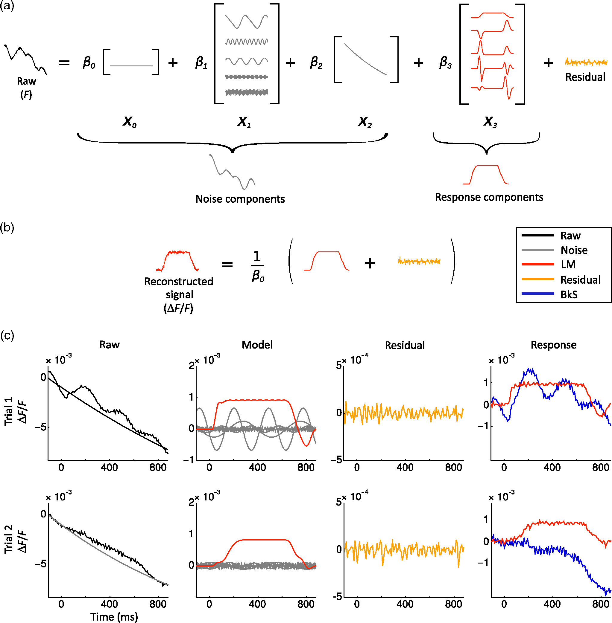

The application of the linear model to two experimental trials in response to a stimulation in the monkey visual cortex is shown in Fig. 4(c). The raw time courses are represented in black in the first column. For each raw signal, the noise components as identified by the model are shown in gray (first column for the bleaching and second column for the periodic components). The evoked response components are shown in red (second column). Bleaching, heartbeat, and fast oscillatory noises were clearly visible on these trials and were well captured by the model. The residuals (mostly white noise) are shown in the third column (orange). The signals, denoised with either the standard blank substraction (blue) or the linear model (red) are shown in the fourth column. As seen in these examples, the linear regression method provides a large improvement in signal to noise.⁶⁹ Further improvement of the method by combining it to convex nonsmooth regularization priors has recently been proposed.⁷⁰

This method thus recovers the signal at single-trial level and offers key data that more faithfully capture the variable population dynamics of cortical networks recorded in VSDI.⁷⁶ Such variability can obsure important spatio-temporal features when averaging VSDI data. In particular, a key question is the question of the spatio-temporal response to small local stimuli. In awake nonhuman primates, spreads of activity have been shown²⁶^,⁶⁹^,⁷⁷ but their origin and the question of whether they represent activity propagation within the cortical tissue have been disputed.⁷⁸^–⁸⁰ Here, our denoising method has enabled us to conclusively answer this debate by applying a new wave detection approach to the data denoised for single-trial analysis. The combination of these LM-denoised data and further signal processing approaches has allowed us to demonstrate that traveling waves are at the origin of the spread emerging at the trial-averaged level.

3.3.

Instantaneous Phase for Revealing Single-Trial Waves

Following denoising of the VSDI signal, further computational approaches are necessary to characterize the complex spatio-temporal dynamics of neocortical networks. In general, these methods aim to quantify spatio-temporal flow of activity in the optical imaging data, often with the goal to characterize propagation of spontaneous and stimulus-evoked waves, a difficult task in the context of the low signal-to-noise ratios commonly encountered when imaging awake behaving animals in vivo. For this task, various computational approaches have been introduced, including the space-frequency singular value decomposition,⁸¹^,⁸² phase-gradient directionality,⁸³ template matching,⁸⁴ and an optic flow-based approach.⁸⁵ In each case, these methods employ a mathematical representation of the optical imaging signal to derive a bounded measure of wave-like organization in the data, allowing to then estimate further quantitative characteristics such as propagation speed, wavelength, and direction. In order to conclusively test whether propagating waves are evoked in the primary visual cortex of the awake monkey in response to small visual stimuli, however, we adopted a statistical approach to wave detection using a phase-based measure.⁸⁶

We first employ the “analytic signal” representation⁸⁷^,⁸⁸ to estimate phase at each pixel in the optical imaging data, as with previous approaches based on this mathematical framework.⁸³ In this representation, a real-valued timeseries [such as values from one pixel of the imaging array; real plane, at bottom, Fig. 5(a)] is transformed into a complex-valued timeseries [line color-coded with increasing heat to indicate time, Fig. 5(a)]. In the complex plane projection [at left, Fig. 5(a)], the result is a “phasor” rotating in the complex plane, whose length (or modulus) represents signal instantaneous amplitude and whose angle (or argument) represents signal instantaneous phase. This estimate of signal phase at each time point can then be used to compare offsets in activity across many pixels, in a manner robust to noisy amplitude fluctuations.

Fig. 5

Phase latency method for detecting waves in single-trial data. (a) The real, imaginary, and complex plane projections of the analytic signal (line colored by heat in time) for a damped oscillation make explicit the decomposition of a real signal into a complex phasor. (b) The complex plane projection in the previous panel is used to analyze instantaneous amplitude ( $A$ , complex modulus) and phase ( $φ$ , complex angle) in the real signal. Gray arrows indicate the direction of phasor rotation in time. The black dot (bottom left) represents the starting point for the phase latency calculation. The blue dots represent discrete samples leading up to the phase crossing. (c) Average phase latency map for the region of interest in the primary visual cortex of awake monkey, in the stimulus (top) and black (bottom) condition. (d) Propagation speeds extracted from the slope of the relation of phase latency with distance in the unsmoothed maps, in the 50-ms stimulus condition. (Inset) Phase latency correlation with distance, stimulus (black) and blank (gray) conditions. Adapted with permission from Ref. 86.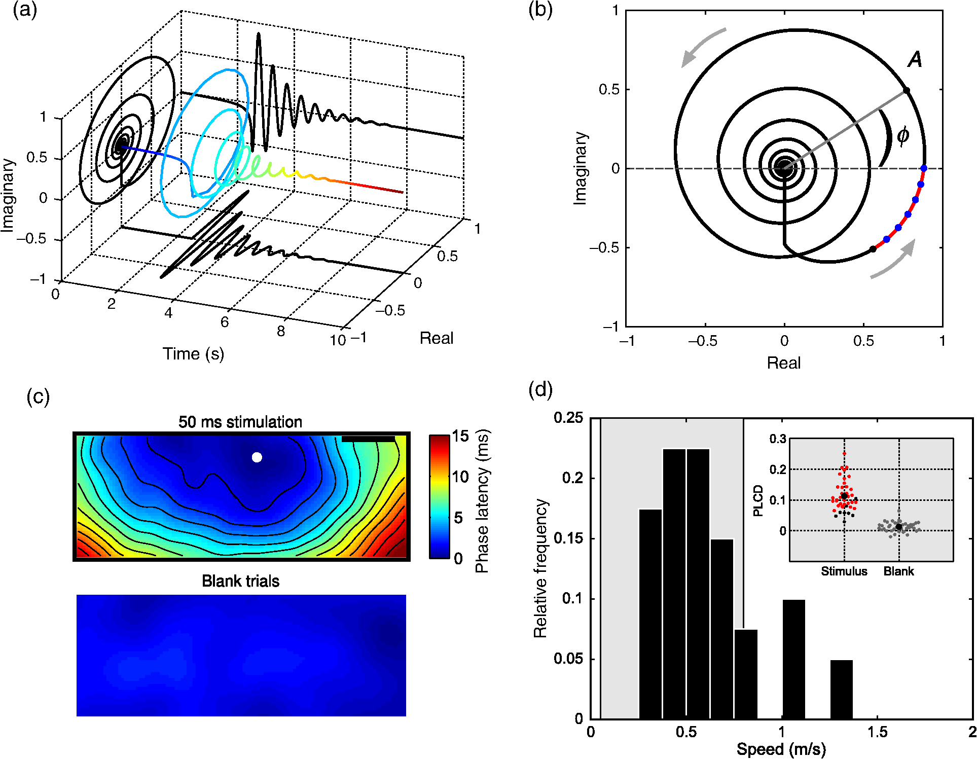

Next, as a signal processing optimization, we introduce a measure termed “phase latency” [red curve, Fig. 5(b)], which quantifies the latency in absolute time to a given phase crossing in the complex plane. Specifically, by starting from a chosen point in the timeseries, for example, a point just before response onset [black dot, Fig. 5(b)], we can calculate the time of the next phase crossing at each pixel. This measure allows us to flexibly compare responses between pixels with slightly differing temporal frequencies, and in this way, it precludes the necessity to filter the data within a tight frequency range. This approach thus has the ultimate effect of reducing overall waveform distortion in the analyzed signal, an important consideration when working with bandpass filtered data. When the phase crossing of interest falls between two discrete samples [blue dots, Fig. 5(b)], the precise time for the crossing is calculated by linear interpolation between the two points based on their instantaneous frequency ( $d φ / d t$ ).

With this measure calculated at each pixel, we then have a “phase latency” map starting from the chosen time point. We next quantify spatial patterns in these maps in several steps. First, we estimate the wave source from the minimum of the smoothed phase latency maps [depicted schematically with a white dot, Fig. 5(c)]. It is important to note here that if the phase latency map contains only noise, without spatiotemporal organization, then the estimated wave source will be at a random point determined by the noise fluctuations. Next, after calculating the Euclidean distance matrix from the source point, we can estimate propagation speed from the slope of the relation of phase latency with distance from the source [Fig. 5(d)] and the correlation coefficient quantifying the strength of this relationship ( $ϱ_{d}$ ). We can then form a well-defined statistical test to determine whether significant phase organization exists in the VSDI data in each trial (one-tailed $t$ -test, $H_{0}$ : $ϱ_{d} = 0$ , $H_{1}$ : $ϱ_{d} > 0$ , in our initial work). Thus, by testing phase organization systematically across all pixels in space, this approach maximizes one of the main strengths of VSDI—its high spatial resolution over a large field-of-view—to enable analysis at the single-trial level. The result of these calculations is a robust and sensitive approach for detecting arbitrarily shaped waves in very high-noise multichannel recordings, by means of a well-defined statistical test.

4. Discussion

In this review, we have provided a series of examples showing that computational approaches can standardize and generalize VSDI as an unmatched tool for studying instantaneous processing by neural circuits. The VSDI signal is indeed unique in the scales and resolutions it reaches (reviewed in Ref. 2) and has already allowed uncovering key dynamic processing and interactions within cortical networks, as shown in particular by Grinvald et al.²⁰^,³⁶^,⁷⁶^,⁸⁹^–⁹¹ The neuronal operations occurring at the mesoscopic scale are still very poorly understood, however, and depart from the dominant feedforward view that usually gives very little credit to horizontal interactions and intracortical processing.⁹²^–⁹⁶ The VSDI signal is complicated and reflects the population membrane potential changes mostly influenced by sub- and not suprathreshold, spiking, activity. We believe that, in addition to the inherent technical difficulties of the method, both the unknown scale and the nonstandard origin of the signal keeps this tool from being used by a majority of researchers in neuroscience systems. However, there is no ideal technique and all existing approaches exhibit methodological drawbacks to be considered. To start with, the gold standard “single-unit activity” must be interpreted with caution since spike identification is never perfect and can be contaminated by neighboring cells, as shown by the literature on spike sorting techniques.⁹⁷^–⁹⁹ At the other end of the recording spectrum, the origin and the link of fMRI signal to neuronal response still remains unclear, even after huge efforts to better understand it through both models and experiment.¹⁰⁰^,¹⁰¹ Similarly, the inverse problem for EEG recordings is still far from being solved despite a lot of computational efforts.¹⁰² Closer to VSDI, two-photon mostly records calcium fluorescence, whose link to spiking activity is nontrivial and needs the development of sophisticated algorithms.¹⁰³^,¹⁰⁴ In all these techniques, computational studies are essential to their development and appropriate use. In this way, the development of VSDI similarly depends on these approaches to fill the gap of our current knowledge on mesoscopic neuronal operations.

On one hand, computational models are, therefore, very important to overcome these hurdles by providing a solid framework to better understand the types of operations subtending the signal’s dynamics and their neuronal origins. Through the close interaction between models and physiology, VSDI data can demonstrate that such operations cannot be summarized in terms of a simple excitatory-inhibitory balance of the feedforward drive.¹⁰⁵ From this perspective, the fact that the signal has a subthreshold origin can be seen as an advantage, since it allows probing the network operations occurring at population level by highlighting their synaptic origin and processing.¹⁰⁶^–¹¹¹ To bridge this gap between network synaptic operations and the mesoscopic population response, computational models are crucial. More generally, theoretical considerations about the information processing and encoding capacities that reside specifically at the mesoscopic scale are clearly needed, both for improving our understanding of the experimental results, but also to generate tractable predictions. Advances in signal processing, on the other hand, are essential to generate standardized and comparable datasets among studies. It is also necessary to remove artifacts that could potentially contaminate the signal and hinder access to analysis of single trials. Since the signal is spatio-temporally inseparable (i.e., cannot be described by two independent spatial and temporal functions), because of inherent propagations due to feedforward and feedback divergence, but also to intracortical connectivity, analyzing data at the single-trial level is essential to understand its dynamics, which are easily corrupted by averaging.⁸⁶^,¹¹²^,¹¹³ Here, computational approaches can help to describe theoretically the type of spatio-temporal dynamics occurring, from single cycle propagating wave, to standing and traveling waves.¹¹⁴

Finally, the inherent methodological difficulties linked to this optical imaging technique have also hindered its development. It is clear that methodological advances such as genetically encoded voltage indicators¹¹⁵^–¹¹⁷ can profoundly help to popularize the technique. However, the theoretical weaknesses linked to our poor understanding of mesoscopic neuronal operations will remain if the computational community does not become more strongly involved. In this review, we have discussed several recent efforts for developing computational methods that have improved our knowledge and understanding of the VSDI signal. However, we believe that there is still a large gap in terms of conceptual framework to interpret and guide the experimental results obtained at this scale. This will only be possible through a closer interactions and collaboration between the physiological and computational communities. Only then, the direction initiated by the remarkable work of Amiram Grinvald will continue to pave the way for understanding the mysteries still hidden at the mesoscopic scale.

Disclosures

The authors have no conflict of interests.

Acknowledgments

This work was supported by the CNRS, the European Community (FET Grant Nos. FACETS FP6-015879, BrainScaleS FP7-269921, and the Human Brain Project H2020-720270 (to AD), the project “BalaV1,” awarded by the Agence Nationale de la Recherche (ANR-13-BSV4-0014-02), and the FRQS Vision Health Research Network of Quebec networking grant. The experimental protocol was approved beforehand by the local Ethical Committee for Animal Research and all procedures complied with the French and European regulations on Animal Research (Approval No. A12/01/13) as well as the guidelines from the Society for Neuroscience.

References

1.

D. Shoham et al., “Imaging cortical dynamics at high spatial and temporal resolution with novel blue voltage-sensitive dyes,” Neuron, 24 (4), 791 –802 (1999). http://dx.doi.org/10.1016/S0896-6273(00)81027-2 NERNET 0896-6273 Google Scholar

2.

A. Grinvald and R. Hildesheim, “VSDI: a new era in functional imaging of cortical dynamics,” Nat. Rev. Neurosci., 5 (11), 874 –885 (2004). http://dx.doi.org/10.1038/nrn1536 NRNAAN 1471-003X Google Scholar

3.

T. J. Sejnowski, P. S. Churchland and J. A. Movshon, “Putting big data to good use in neuroscience,” Nat. Neurosci., 17 (11), 1440 –1441 (2014). http://dx.doi.org/10.1038/nn.3839 Google Scholar

4.

N. T. Markov et al., “Weight consistency specifies regularities of macaque cortical networks,” Cerebral Cortex, 21 (6), 1254 –1272 (2011). http://dx.doi.org/10.1093/cercor/bhq201 Google Scholar

5.

O. Faugeras, J. Touboul and B. Cessac, “A constructive mean-field analysis of multi-population neural networks with random synaptic weights and stochastic inputs,” Front. Comput. Neurosci., 3 1 (2009). http://dx.doi.org/10.3389/neuro.10.001.2009 1662-5188 Google Scholar

6.

J.-L. R. Stevens et al., “Mechanisms for stable, robust, and adaptive development of orientation maps in the primary visual cortex,” J. Neurosci., 33 (40), 15747 –15766 (2013). http://dx.doi.org/10.1523/JNEUROSCI.1037-13.2013 JNRSDS 0270-6474 Google Scholar

7.

C. La Rota, Analyse de l’activité électrique multi-sites du cortex auditif chez le cobaye, Université Joseph Fourier, Grenoble (2003). Google Scholar

8.

A. V. Rangan, D. Cai and D. W. McLaughlin, “Modeling the spatiotemporal cortical activity associated with the line-motion illusion in primary visual cortex,” Proc. Natl. Acad. Sci. U.S.A., 102 (52), 18793 –18800 (2005). http://dx.doi.org/10.1073/pnas.0509481102 PNASA6 0027-8424 Google Scholar

9.

Y. Sit and R. Miikkulainen, “A computational model of the signals in optical imaging with voltage-sensitive dyes,” Neurocomputing, 70 (10–12), 1853 –1857 (2007). http://dx.doi.org/10.1016/j.neucom.2006.10.089 NRCGEO 0925-2312 Google Scholar

10.

F. Grimbert and F. Chavane, “Neural field model of VSD optical imaging signals,” (2007). Google Scholar

11.

S. El Boustani and A. Destexhe, “A master equation formalism for macroscopic modeling of asynchronous irregular activity states,” Neural Comput., 21 (1), 46 –100 (2009). http://dx.doi.org/10.1162/neco.2009.02-08-710 NEUCEB 0899-7667 Google Scholar

12.

A. Symes and T. Wennekers, “Spatiotemporal dynamics in the cortical microcircuit: a modelling study of primary visual cortex layer 2/3,” Neural Networks, 22 (8), 1079 –1092 (2009). http://dx.doi.org/10.1016/j.neunet.2009.07.017 NNETEB 0893-6080 Google Scholar

13.

V. Markounikau et al., “A dynamic neural field model of mesoscopic cortical activity captured with voltage-sensitive dye imaging,” PLoS Comput. Biol., 6 (9), e1000919 (2010). http://dx.doi.org/10.1371/journal.pcbi.1000919.t001 Google Scholar

14.

G. Deco and P. Roland, “The role of multi-area interactions for the computation of apparent motion,” NeuroImage, 51 (3), 1018 –1026 (2010). http://dx.doi.org/10.1016/j.neuroimage.2010.03.032 NEIMEF 1053-8119 Google Scholar

15.

A. V. Chizhov, “Conductance-based refractory density model of primary visual cortex,” J. Comput. Neurosci., 36 (2), 297 –319 (2014). http://dx.doi.org/10.1007/s10827-013-0473-5 JCNEFR 0929-5313 Google Scholar

16.

H. R. Wilson and J. D. Cowan, “Excitatory and inhibitory interactions in localized populations of model neurons,” Biophys. J., 12 (1), 1 –24 (1972). http://dx.doi.org/10.1016/S0006-3495(72)86068-5 BIOJAU 0006-3495 Google Scholar

17.

J. Sirosh and R. Miikkulainen, “Cooperative self-organization of afferent and lateral connections in cortical maps,” Biol. Cybern., 71 65 –78 (1994). http://dx.doi.org/10.1007/BF00198912 BICYAF 0340-1200 Google Scholar

18.

R. Miikkulainen et al., Computational Maps in the Visual Cortex, Springer, New York (2005). Google Scholar

19.

T. Kohonen, Self-Organizing Maps, Springer, Berlin, Germany (2001). Google Scholar

20.

D. Jancke et al., “Imaging cortical correlates of illusion in early visual cortex,” Nature, 428 (6981), 423 –426 (2004). http://dx.doi.org/10.1038/nature02396 Google Scholar

21.

A. Destexhe, “Conductance-based integrate-and-fire models,” Neural Comput., 9 (3), 503 –514 (1997). http://dx.doi.org/10.1162/neco.1997.9.3.503 NEUCEB 0899-7667 Google Scholar

22.

B. Ahmed et al., “Cortical dynamics subserving visual apparent motion,” Cerebral Cortex, 18 (12), 2796 –2810 (2008). http://dx.doi.org/10.1093/cercor/bhn038 Google Scholar

23.

S. Chemla and F. Chavane, “A biophysical cortical column model to study the multi-component origin of the VSDI signal,” NeuroImage, 53 (2), 420 –438 (2010). http://dx.doi.org/10.1016/j.neuroimage.2010.06.026 NEIMEF 1053-8119 Google Scholar

24.

D. Cai, A. V. Rangan and D. W. McLaughlin, “Architectural and synaptic mechanisms underlying coherent spontaneous activity in V1,” Proc. Natl. Acad. Sci. U.S.A., 102 (16), 5868 –5873 (2005). http://dx.doi.org/10.1073/pnas.0501913102 PNASA6 0027-8424 Google Scholar

25.

H. S. Orbach and L. B. Cohen, “Optical monitoring of activity from many areas of the in vitro and in vivo salamander olfactory bulb: a new method for studying functional organization in the vertebrate central nervous system,” J. Neurosci., 3 (11), 2251 –2262 (1983). JNRSDS 0270-6474 Google Scholar

26.

A. Reynaud, G. S. Masson and F. Chavane, “Dynamics of local input normalization result from balanced short- and long-range intracortical interactions in area V1,” J. Neurosci., 32 (36), 12558 –12569 (2012). http://dx.doi.org/10.1523/JNEUROSCI.1618-12.2012 JNRSDS 0270-6474 Google Scholar

27.

A. Reynaud et al., “Input-output transformation in the visuo-oculomotor loop: comparison of real-time optical imaging recordings in V1 to ocular following responses upon center-surround stimulation,” Arch. Ital. Biol., 145 (3–4), 251 –262 (2007). AIBLAS 0003-9829 Google Scholar

28.

L. G. Nowak et al., “Electrophysiological classes of cat primary visual cortical neurons in vivo as revealed by quantitative analyses,” J. Neurophysiol., 89 (3), 1541 –1566 (2003). http://dx.doi.org/10.1152/jn.00580.2002 JONEA4 0022-3077 Google Scholar

29.

T. Binzegger, “A quantitative map of the circuit of cat primary visual cortex,” J. Neurosci., 24 (39), 8441 –8453 (2004). http://dx.doi.org/10.1523/JNEUROSCI.1400-04.2004 JNRSDS 0270-6474 Google Scholar

30.

D. Contreras and L. Palmer, “Response to contrast of electrophysiologically defined cell classes in primary visual cortex,” J. Neurosci., 23 (17), 6936 –6945 (2003). JNRSDS 0270-6474 Google Scholar

31.

P. Buzás et al., “Axonal topography of cortical basket cells in relation to orientation, direction, and ocular dominance maps,” J. Comput. Neurol., 437 (3), 259 –285 (2001). Google Scholar

32.

P. Buzás et al., “Model-based analysis of excitatory lateral connections in the visual cortex,” J. Comput. Neurol., 499 (6), 861 –881 (2006). http://dx.doi.org/10.1002/(ISSN)1096-9861 Google Scholar

33.

A. Destexhe et al., “Fluctuating synaptic conductances recreate in vivo-like activity in neocortical neurons,” Neuroscience, 107 (1), 13 –24 (2001). Google Scholar

34.

M. T. Lippert et al., “Methods for voltage-sensitive dye imaging of rat cortical activity with high signal-to-noise ratio,” J. Neurophysiol., 98 (1), 502 –512 (2007). http://dx.doi.org/10.1152/jn.01169.2006 JONEA4 0022-3077 Google Scholar

35.

S. Chemla and F. Chavane, “Effects of GABAA kinetics on cortical population activity: computational studies and physiological confirmations,” J. Neurophysiol., 115 2867 –2879 (2016). http://dx.doi.org/10.1152/jn.00352.2015 JONEA4 0022-3077 Google Scholar

36.

D. Sharon and A. Grinvald, “Dynamics and constancy in cortical spatiotemporal patterns of orientation processing,” Science, 295 (5554), 512 –515 (2002). http://dx.doi.org/10.1126/science.1065916 SCIEAS 0036-8075 Google Scholar

37.

V. Kozyrev, U. T. Eysel and D. Jancke, “Voltage-sensitive dye imaging of transcranial magnetic stimulation-induced intracortical dynamics,” Proc. Natl. Acad. Sci. U.S.A., 111 (37), 13553 –13558 (2014). http://dx.doi.org/10.1073/pnas.1405508111 Google Scholar

38.

S. Onat et al., “Independent encoding of grating motion across stationary feature maps in primary visual cortex visualized with voltage-sensitive dye imaging,” NeuroImage, 55 (4), 1763 –1770 (2011). http://dx.doi.org/10.1016/j.neuroimage.2011.01.004 NEIMEF 1053-8119 Google Scholar

39.

G. G. Blasdel, “Differential imaging of ocular dominance and orientation selectivity in monkey striate cortex,” J. Neurosci., 12 (8), 3115 –3138 (1992). JNRSDS 0270-6474 Google Scholar

40.

A. Grinvald et al., “In-vivo optical imaging of cortical architecture and dynamics,” Mod. Technol. Neurosci. Res., 91 893 –969 (1999). http://dx.doi.org/10.1007/978-3-642-58552-4_34 Google Scholar

41.

S. Chakraborty, A. Sandberg and S. A. Greenfield, “Differential dynamics of transient neuronal assemblies in visual compared to auditory cortex,” Exp. Brain Res., 182 (4), 491 –498 (2007). http://dx.doi.org/10.1007/s00221-007-1008-y EXBRAP 0014-4819 Google Scholar

42.

Y. Chen, W. S. Geisler and E. Seidemann, “Optimal temporal decoding of neural population responses in a reaction-time visual detection task,” J. Neurophysiol., 99 (3), 1366 –1379 (2008). http://dx.doi.org/10.1152/jn.00698.2007 JONEA4 0022-3077 Google Scholar

43.

S. Roux et al., “Probing the functional impact of sub-retinal prosthesis,” Elife, 5 e12687 (2016). http://dx.doi.org/10.7554/eLife.12687 Google Scholar

44.

K. Takagaki et al., “Normalization of voltage-sensitive dye signal with functional activity measures,” PLoS One, 3 (12), e4041 (2008). http://dx.doi.org/10.1371/journal.pone.0004041.g008 POLNCL 1932-6203 Google Scholar

45.

R. A. Carmona, W. L. Hwang and R. D. Frostig, “Wavelet analysis for brain-function imaging,” IEEE Trans. Med. Imaging, 14 (3), 556 –564 (1995). http://dx.doi.org/10.1109/42.414621 ITMID4 0278-0062 Google Scholar

46.

A. F. Cannestra et al., “The evolution of optical signals in human and rodent cortex,” NeuroImage, 3 (3 Pt 1), 202 –208 (1996). http://dx.doi.org/10.1006/nimg.1996.0022 NEIMEF 1053-8119 Google Scholar

47.

A. Sornborger et al., “Spatiotemporal analysis of optical imaging data,” NeuroImage, 18 (3), 610 –621 (2003). http://dx.doi.org/10.1016/S1053-8119(02)00045-9 NEIMEF 1053-8119 Google Scholar

48.

M. Stetter, “Principal component analysis and blind separation of sources for optical imaging of intrinsic signals,” NeuroImage, 11 (5), 482 –490 (2000). http://dx.doi.org/10.1006/nimg.2000.0551 NEIMEF 1053-8119 Google Scholar

49.

I. Schiessl, W. Wang and N. McLoughlin, “Independent components of the haemodynamic response in intrinsic optical imaging,” NeuroImage, 39 (2), 634 –646 (2008). http://dx.doi.org/10.1016/j.neuroimage.2007.09.022 NEIMEF 1053-8119 Google Scholar

50.

R. Everson, B. W. Knight and L. Sirovich, “Separating spatially distributed response to stimulation from background. I. Optical imaging,” Biol. Cybern., 77 (6), 407 –417 (1997). http://dx.doi.org/10.1007/s004220050400 BICYAF 0340-1200 Google Scholar

51.

M. Gabbay, “A principal components-based method for the detection of neuronal activity maps: application to optical imaging,” NeuroImage, 11 (4), 313 –325 (2000). http://dx.doi.org/10.1006/nimg.2000.0547 NEIMEF 1053-8119 Google Scholar

52.

T. Yokoo, “An optimization approach to signal extraction from noisy multivariate data,” NeuroImage, 14 (6), 1309 –1326 (2001). http://dx.doi.org/10.1006/nimg.2001.0950 NEIMEF 1053-8119 Google Scholar

53.

G. D. Brown, S. Yamada and T. J. Sejnowski, “Independent component analysis at the neural cocktail party,” Trends Neurosci., 24 (1), 54 –63 (2001). http://dx.doi.org/10.1016/S0166-2236(00)01683-0 TNSCDR 0166-2236 Google Scholar

54.

S. Maeda et al., “Separation of signal and noise from in vivo optical recording in Guinea pigs using independent component analysis,” Neurosci. Lett., 302 (2–3), 137 –140 (2001). http://dx.doi.org/10.1016/S0304-3940(01)01678-0 NELED5 0304-3940 Google Scholar

55.

S. Inagaki et al., “Isolation of neural activities from respiratory and heartbeat noises for in vivo optical recording in guinea pigs using independent component analysis,” Neurosci. Lett., 352 (1), 9 –12 (2003). NELED5 0304-3940 Google Scholar

56.

Y. Zheng et al., “Signal source separation in the analysis of neural activity in brain,” NeuroImage, 13 (3), 447 –458 (2001). http://dx.doi.org/10.1006/nimg.2000.0705 NEIMEF 1053-8119 Google Scholar

57.

J. Reidl et al., “Independent component analysis of high-resolution imaging data identifies distinct functional domains,” NeuroImage, 34 (1), 94 –108 (2007). http://dx.doi.org/10.1016/j.neuroimage.2006.08.031 NEIMEF 1053-8119 Google Scholar

58.

T. Fekete et al., “Removal of spatial biological artifacts in functional maps by local similarity minimization,” J. Neurosci. Methods, 178 (1), 31 –39 (2009). http://dx.doi.org/10.1016/j.jneumeth.2008.11.020 JNMEDT 0165-0270 Google Scholar

59.

D. B. Omer, R. Hildesheim and A. Grinvald, “Temporally-structured acquisition of multidimensional optical imaging data facilitates visualization of elusive cortical representations in the behaving monkey,” NeuroImage, 82 237 –251 (2013). http://dx.doi.org/10.1016/j.neuroimage.2013.05.045 NEIMEF 1053-8119 Google Scholar

60.

E. S. Hill et al., “Validation of independent component analysis for rapid spike sorting of optical recording data,” J. Neurophysiol., 104 (6), 3721 –3731 (2010). http://dx.doi.org/10.1152/jn.00691.2010 JONEA4 0022-3077 Google Scholar

61.

S. A. Engel et al., “fMRI of human visual cortex,” Nature, 369 (6481), 525 (1994). http://dx.doi.org/10.1038/369525a0 Google Scholar

62.

V. A. Kalatsky and M. P. Stryker, “New paradigm for optical imaging: temporally encoded maps of intrinsic signal,” Neuron, 38 (4), 529 –545 (2003). http://dx.doi.org/10.1016/S0896-6273(03)00286-1 NERNET 0896-6273 Google Scholar

63.

Z. Yang, D. J. Heeger and E. Seidemann, “Rapid and precise retinotopic mapping of the visual cortex obtained by voltage-sensitive dye imaging in the behaving monkey,” J. Neurophysiol., 98 (2), 1002 –1014 (2007). http://dx.doi.org/10.1152/jn.00417.2007 JONEA4 0022-3077 Google Scholar

64.

K. J. Friston, A. P. Holmes and K. J. Worsley, “Statistical parametric maps in functional imaging: a general linear approach,” Hum. Brain, 2 189 –210 (1994). http://dx.doi.org/10.1002/hbm.460020402 Google Scholar

65.

D. Rector, “Scattered-light imaging in vivo tracks fast and slow processes of neurophysiological activation,” NeuroImage, 14 (5), 977 –994 (2001). http://dx.doi.org/10.1006/nimg.2001.0897 NEIMEF 1053-8119 Google Scholar

66.

B. Bathellier et al., “Wavelet-based multi-resolution statistics for optical imaging signals: application to automated detection of odour activated glomeruli in the mouse olfactory bulb,” NeuroImage, 34 (3), 1020 –1035 (2007). http://dx.doi.org/10.1016/j.neuroimage.2006.10.038 NEIMEF 1053-8119 Google Scholar

67.

J. Mayhew et al., “An evaluation of linear model analysis techniques for processing images of microcirculation activity,” NeuroImage, 7 (1), 49 –71 (1998). http://dx.doi.org/10.1006/nimg.1997.0311 NEIMEF 1053-8119 Google Scholar

68.

M. Stetter, “Analysis of calcium imaging signals from the honeybee brain by nonlinear models,” NeuroImage, 13 (1), 119 –128 (2001). http://dx.doi.org/10.1006/nimg.2000.0679 NEIMEF 1053-8119 Google Scholar

69.

A. Reynaud et al., “Linear model decomposition for voltage-sensitive dye imaging signals: application in awake behaving monkey,” NeuroImage, 54 (2), 1196 –1210 (2011). http://dx.doi.org/10.1016/j.neuroimage.2010.08.041 NEIMEF 1053-8119 Google Scholar

70.

H. Raguet et al., “Spatially structured sparse morphological component separation for voltage-sensitive dye optical imaging,” J. Neurosci. Method, 257 76 –96 (2016). http://dx.doi.org/10.1016/j.jneumeth.2015.09.024 JNMEDT 0165-0270 Google Scholar

71.

G.-A. Hossein-Zadeh, B. A. Ardekani and H. Soltanian-Zadeh, “A signal subspace approach for modeling the hemodynamic response function in fMRI,” Magn. Reson Imaging, 21 (8), 835 –843 (2003). Google Scholar

72.

M. W. Woolrich, T. Behrens and S. M. Smith, “Constrained linear basis sets for HRF modelling using variational Bayes,” NeuroImage, 21 1748 –1761 (2004). http://dx.doi.org/10.1016/j.neuroimage.2003.12.024 NEIMEF 1053-8119 Google Scholar

73.

S. Takerkart et al., “Vobi One: a data processing software package for functional optical imaging,” Front. Neurosci., 8 2 (2014). http://dx.doi.org/10.3389/fnins.2014.00002 1662-453X Google Scholar

74.

P. E. Williams et al., “Entrainment to video displays in primary visual cortex of macaque and humans,” J. Neurosci., 24 (38), 8278 –8288 (2004). http://dx.doi.org/10.1523/JNEUROSCI.2716-04.2004 JNRSDS 0270-6474 Google Scholar

75.

A. Grinvald et al., “Cortical point-spread function and long-range lateral interactions revealed by real-time optical imaging of macaque monkey primary visual cortex,” J. Neurosci., 14 (5 Pt 1), 2545 –2568 (1994). JNRSDS 0270-6474 Google Scholar

76.

A. Arieli et al., “Dynamics of ongoing activity: explanation of the large variability in evoked cortical responses,” Science, 273 (5283), 1868 –1871 (1996). SCIEAS 0036-8075 Google Scholar

77.

H. Slovin et al., “Long-term voltage-sensitive dye imaging reveals cortical dynamics in behaving monkeys,” J. Neurophysiol., 88 (6), 3421 –3438 (2002). http://dx.doi.org/10.1152/jn.00194.2002 JONEA4 0022-3077 Google Scholar

78.

Y. F. Sit et al., “Complex dynamics of V1 population responses explained by a simple gain-control model,” Neuron, 64 (6), 943 –956 (2009). http://dx.doi.org/10.1016/j.neuron.2009.08.041 NERNET 0896-6273 Google Scholar

79.

S. Ray and J. H. R. Maunsell, “Different origins of gamma rhythm and high-gamma activity in macaque visual cortex,” PLoS Biol., 9 (4), e1000610 (2011). http://dx.doi.org/10.1371/journal.pbio.1000610.g008 Google Scholar

80.

I. Nauhaus et al., “Robustness of traveling waves in ongoing activity of visual cortex,” J. Neurosci., 32 (9), 3088 –3094 (2012). http://dx.doi.org/10.1523/JNEUROSCI.5827-11.2012 JNRSDS 0270-6474 Google Scholar

81.

J. C. Prechtl, L. B. Cohen and B. Pesaran, “Visual stimuli induce waves of electrical activity in turtle cortex,” Proc. Natl. Acad. Sci. U.S.A., 94 7621 –7626 (1997). Google Scholar

82.

P. P. Mitra and B. Pesaran, “Analysis of dynamic brain imaging data,” Biophys. J., 76 (2), 691 –708 (1999). http://dx.doi.org/10.1016/S0006-3495(99)77236-X BIOJAU 0006-3495 Google Scholar

83.

D. Rubino, K. A. Robbins and N. G. Hatsopoulos, “Propagating waves mediate information transfer in the motor cortex,” Nat. Neurosci., 9 (12), 1549 –1557 (2006). http://dx.doi.org/10.1038/nn1802 NANEFN 1097-6256 Google Scholar

84.

K. Takagaki et al., “Flow detection of propagating waves with temporospatial correlation of activity,” J. Neurosci. Methods, 200 207 –218 (2011). http://dx.doi.org/10.1016/j.jneumeth.2011.05.023 JNMEDT 0165-0270 Google Scholar

85.

M. H. Mohajerani et al., “Spontaneous cortical activity alternates between motifs defined by regional axonal projections,” Nat. Res., 16 (10), 1426 –1435 (2013). http://dx.doi.org/10.1038/nn.3499 Google Scholar

86.

L. Muller et al., “The stimulus-evoked population response in visual cortex of awake monkey is a propagating wave,” Nat. Commun., 5 3675 (2014). http://dx.doi.org/10.1038/ncomms4675 NCAOBW 2041-1723 Google Scholar

87.

D. Gabor, “Theory of communication. Part 1: the analysis of information,” J. Inst. Elect. Eng., 93 429 –441 (1946). http://dx.doi.org/10.1049/ji-3-2.1946.0074 Google Scholar

88.

M. Feldman, Hilbert Transform Applications in Mechanical Vibration, John Wiley & Sons, Hoboken, New Jersey (2011). Google Scholar

89.

T. Kenet et al., “Spontaneously emerging cortical representations of visual attributes,” Nature, 425 (6961), 954 –956 (2003). http://dx.doi.org/10.1038/nature02078 Google Scholar

90.

F. Chavane et al., “Lateral spread of orientation selectivity in V1 is controlled by intracortical cooperativity,” Front. Syst. Neurosci., 5 4 (2011). http://dx.doi.org/10.3389/fnsys.2011.00004 Google Scholar

91.

E. Seidemann et al., “Dynamics of depolarization and hyperpolarization in the frontal cortex and saccade goal,” Science, 295 (5556), 862 –865 (2002). http://dx.doi.org/10.1126/science.1066641 SCIEAS 0036-8075 Google Scholar

92.

V. A. Lamme and P. R. Roelfsema, “The distinct modes of vision offered by feedforward and recurrent processing,” Trends Neurosci., 23 (11), 571 –579 (2000). http://dx.doi.org/10.1016/S0166-2236(00)01657-X TNSCDR 0166-2236 Google Scholar

93.

N. C. Rust et al., “How MT cells analyze the motion of visual patterns,” Nat. Neurosci., 9 (11), 1421 –1431 (2006). http://dx.doi.org/10.1038/nn1786 NANEFN 1097-6256 Google Scholar

94.

J. J. DiCarlo, D. Zoccolan and N. C. Rust, “How does the brain solve visual object recognition?,” Neuron, 73 (3), 415 –434 (2012). http://dx.doi.org/10.1016/j.neuron.2012.01.010 NERNET 0896-6273 Google Scholar

95.

J. Bullier, “Integrated model of visual processing,” Brain Res. Rev., 36 (2–3), 96 –107 (2001). BRERD2 0165-0173 Google Scholar

96.

T. Serre, A. Oliva and T. Poggio, “A feedforward architecture accounts for rapid categorization,” Proc. Natl. Acad. Sci. U.S.A., 104 (15), 6424 –6429 (2007). http://dx.doi.org/10.1073/pnas.0700622104 PNASA6 0027-8424 Google Scholar

97.

G. T. Einevoll et al., “Towards reliable spike-train recordings from thousands of neurons with multielectrodes,” Curr. Opin. Neurobiol., 22 (1), 11 –17 (2012). http://dx.doi.org/10.1016/j.conb.2011.10.001 COPUEN 0959-4388 Google Scholar

98.

H. G. Rey, C. Pedreira and R. Quian Quiroga, “Past, present and future of spike sorting techniques,” Brain Res. Bull., 119 (Pt. B), 106 –117 (2015). http://dx.doi.org/10.1016/j.brainresbull.2015.04.007 BRBUDU 0361-9230 Google Scholar

99.

K. D. Harris et al., “Improving data quality in neuronal population recordings,” Nat. Neurosci., 19 1165 –1174 (2016). http://dx.doi.org/10.1038/nn.4365 NANEFN 1097-6256 Google Scholar

100.

D. J. Heeger and D. Ress, “What does FMRI tell us about neuronal activity?,” Nat. Rev. Neurosci., 3 (2), 142 –151 (2002). http://dx.doi.org/10.1038/nrn730 NRNAAN 1471-003X Google Scholar

101.

R. B. Buxton, “Dynamic models of BOLD contrast,” NeuroImage, 62 (2), 953 –961 (2012). http://dx.doi.org/10.1016/j.neuroimage.2012.01.012 NEIMEF 1053-8119 Google Scholar

102.

R. Grech et al., “Review on solving the inverse problem in EEG source analysis,” J. Neuroeng. Rehabil., 5 25 (2008). http://dx.doi.org/10.1186/1743-0003-5-25 Google Scholar

103.

T. Deneux et al., “Accurate spike estimation from noisy calcium signals for ultrafast three-dimensional imaging of large neuronal populations in vivo,” Nat. Commun., 7 1 –17 (2016). http://dx.doi.org/10.1038/ncomms12190 NCAOBW 2041-1723 Google Scholar

104.

S. R. Schultz et al., “Advances in two-photon scanning and scanless microscopy technologies for functional neural circuit imaging,” Proc. IEEE, 105 (1), 139 –157 (2017). http://dx.doi.org/10.1109/JPROC.2016.2577380 IEEPAD 0018-9219 Google Scholar

105.

K. D. Miller, “Understanding layer 4 of the cortical circuit: a model based on Cat V1,” Cerebral Cortex, 13 (1), 73 –82 (2003). http://dx.doi.org/10.1093/cercor/13.1.73 Google Scholar

106.

R. J. Douglas and K. A. Martin, “A functional microcircuit for cat visual cortex,” J. Physiol., 440 735 –769 (1991). JPHYA7 0022-3751 Google Scholar

107.

V. Bringuier et al., “Horizontal propagation of visual activity in the synaptic integration field of area 17 neurons,” Science, 283 (5402), 695 –699 (1999). http://dx.doi.org/10.1126/science.283.5402.695 SCIEAS 0036-8075 Google Scholar

108.

L. J. Borg-Graham, C. Monier and Y. Frégnac, “Visual input evokes transient and strong shunting inhibition in visual cortical neurons,” Nature, 393 (6683), 369 –373 (1998). http://dx.doi.org/10.1038/30735 Google Scholar

109.

M. Carandini and D. Ferster, “Membrane potential and firing rate in cat primary visual cortex,” J. Neurosci., 20 (1), 470 –484 (2000). JNRSDS 0270-6474 Google Scholar

110.

C. Monier et al., “Orientation and direction selectivity of synaptic inputs in visual cortical neurons: a diversity of combinations produces spike tuning,” Neuron, 37 (4), 663 –680 (2003). http://dx.doi.org/10.1016/S0896-6273(03)00064-3 NERNET 0896-6273 Google Scholar

111.

N. J. Priebe and D. Ferster, “Mechanisms of neuronal computation in mammalian visual cortex,” Neuron, 75 (2), 194 –208 (2012). http://dx.doi.org/10.1016/j.neuron.2012.06.011 NERNET 0896-6273 Google Scholar

112.

W. Xu et al., “Compression and reflection of visually evoked cortical waves,” Neuron, 55 (1), 119 –129 (2007). http://dx.doi.org/10.1016/j.neuron.2007.06.016 NERNET 0896-6273 Google Scholar

113.

D. M. Alexander et al., “Traveling waves and trial averaging: the nature of single-trial and averaged brain responses in large-scale cortical signals,” NeuroImage, 73 95 –112 (2013). http://dx.doi.org/10.1016/j.neuroimage.2013.01.016 NEIMEF 1053-8119 Google Scholar

114.

A. Benucci, R. Frazor and M. Carandini, “Standing waves and traveling waves distinguish two circuits in visual cortex,” Neuron, 55 (1), 103 –117 (2007). http://dx.doi.org/10.1016/j.neuron.2007.06.017 NERNET 0896-6273 Google Scholar

115.

Y. Gong et al., “High-speed recording of neural spikes in awake mice and flies with a fluorescent voltage sensor,” Science, 350 (6266), 1361 –1366 (2015). http://dx.doi.org/10.1126/science.aab0810 SCIEAS 0036-8075 Google Scholar

116.

M. Carandini et al., “Imaging the awake visual cortex with a genetically encoded voltage indicator,” J. Neurosci., 35 (1), 53 –63 (2015). http://dx.doi.org/10.1523/JNEUROSCI.0594-14.2015 JNRSDS 0270-6474 Google Scholar

117.

H. H. Yang and F. St-Pierre, “Genetically encoded voltage indicators: opportunities and challenges,” J. Neurosci., 36 (39), 9977 –9989 (2016). http://dx.doi.org/10.1523/JNEUROSCI.1095-16.2016 JNRSDS 0270-6474 Google Scholar

Biography

Sandrine Chemla received an engineer diploma in microelectronics in 2005. She then have followed a true interdisciplinary track, starting with a PhD in computational neuroscience in 2010, developing a model of the voltage-sensitive dye imaging (University of Sophia-Antipolis, France), followed by a postdoctoral research using VSDI in various species, from the rodent (Lethbridge University, Canada) to the awake nonhuman primate (INT, Marseille, France), with a specific focus on the spatio-temporal cortical dynamics of sensory processing.

Lyle Muller is a postdoctoral fellow in the Computational Neurobiology Laboratory (CNL) at the Salk Institute for Biological Studies. After studying at Brown University (ScB) and Université Pierre et Marie Curie (PhD), he now pursues research in signal processing, computational neuroscience, and graph theory for analysis and modeling of large-scale network dynamics in cortex. Supplementary scientific materials, including links to open-access software releases, are available at his homepage: http://cnl.salk.edu/~lmuller.

Alexandre Reynaud received a computer science engineer diploma from the Polytech'Sophia School and a master's degree in applied image processing at the Université de Nice Sophia-Antipolis in 2005. He completed a PhD in neurosciences in Aix-Marseille Université, which main topic was the study of lateral interactions in macaque primary visual cortex with voltage-sensitive dye imaging. Since 2011, he is working as a post-doc and then as a research associate in McGill University, studying binocular combination.

Sylvain Takerkart has been a reasearch engineer at the French “Centre National pour la Recherche Scientifique” since 2006. At present, he is coordinating the Computing Center of the Institut de Neurosciences de la Timone in Marseilles, France. His research activities focus on developing machine learning tools for image processing problems encountered in neuroscience, with a particular emphasis on the understanding of interindividual variability.

Alain Destexhe is research director at the CNRS and leads a group of computational neuroscience at the UNIC, in the CNRS campus of Gif sur Yvette. He is also director of the European Institute for Theoretical Neuroscience (www.eitn.org) in Paris. He published more than 130 articles in peer-reviewed journals, two monographs and wrote many reviews and book chapters. He is in the editorial board of seven journals in the field of neuroscience and computational neuroscience.

Frédéric Chavane is research director at the CNRS and leads the group “Inference and Visual Behavior” at INT, Marseille, France. He is also codirector of the PhD program in neurosciences of Aix-Marseille University. His main research interest focuses on the role of cortico-cortical dynamical interactions in visual processing, using in particular voltage-sensitive dye imaging in awake nonhuman primates. His research aims at understanding the theoretical underpinnings of neuronal computations subtending dynamical representations within cortical maps.

CC BY: © The Authors. Published by SPIE under a Creative Commons Attribution 4.0 Unported License. Distribution or reproduction of this work in whole or in part requires full attribution of the original publication, including its DOI.

Citation Download Citation

Sandrine Chemla, Lyle Muller, Alexandre Reynaud, Sylvain Takerkart, Alain Destexhe, and Frédéric Chavane "Improving voltage-sensitive dye imaging: with a little help from computational approaches," Neurophotonics 4(3), 031215 (19 May 2017). https://doi.org/10.1117/1.NPh.4.3.031215

Received: 20 January 2017; Accepted: 24 April 2017; Published: 19 May 2017

Access the abstract

JOURNAL ARTICLE
12 PAGES

DOWNLOAD PAPER SAVE TO MY LIBRARY

GET CITATION

CITATIONS

Cited by 27 scholarly publications.

Explore citations on Lens.org

KEYWORDS

Voltage sensitive dyes

Brain

Bridges

In vitro testing

Molecular bridges

Neuroimaging

Neuroscience

1.

Introduction