Review of mesoscopic optical tomography for depth-resolved imaging of hemodynamic changes and neural activities

Qinggong Tang; Jonathan Lin; Vassiliy Tsytsarev; Reha S. Erzurumlu; Yi Liu; Yu Chen

doi:10.1117/1.NPh.4.1.011009

14 November 2016 Review of mesoscopic optical tomography for depth-resolved imaging of hemodynamic changes and neural activities

Qinggong Tang, Jonathan Lin, Vassiliy Tsytsarev, Reha S. Erzurumlu, Yi Liu, Yu Chen

Author Affiliations +

Neurophotonics, Vol. 4, Issue 1, 011009 (November 2016). https://doi.org/10.1117/1.NPh.4.1.011009

Abstract

Understanding the functional wiring of neural circuits and their patterns of activation following sensory stimulations is a fundamental task in the field of neuroscience. Furthermore, charting the activity patterns is undoubtedly important to elucidate how neural networks operate in the living brain. However, optical imaging must overcome the effects of light scattering in the tissue, which limit the light penetration depth and affect both the imaging quantitation and sensitivity. Laminar optical tomography (LOT) is a three-dimensional (3-D) in-vivo optical imaging technique that can be used for functional imaging. LOT can achieve both a resolution of 100 to 200 μm and a penetration depth of 2 to 3 mm based either on absorption or fluorescence contrast, as well as large field-of-view and high acquisition speed. These advantages make LOT suitable for 3-D depth-resolved functional imaging of the neural functions in the brain and spinal cords. We review the basic principles and instrumentations of representative LOT systems, followed by recent applications of LOT on 3-D imaging of neural activities in the rat forepaw stimulation model and mouse whisker-barrel system.

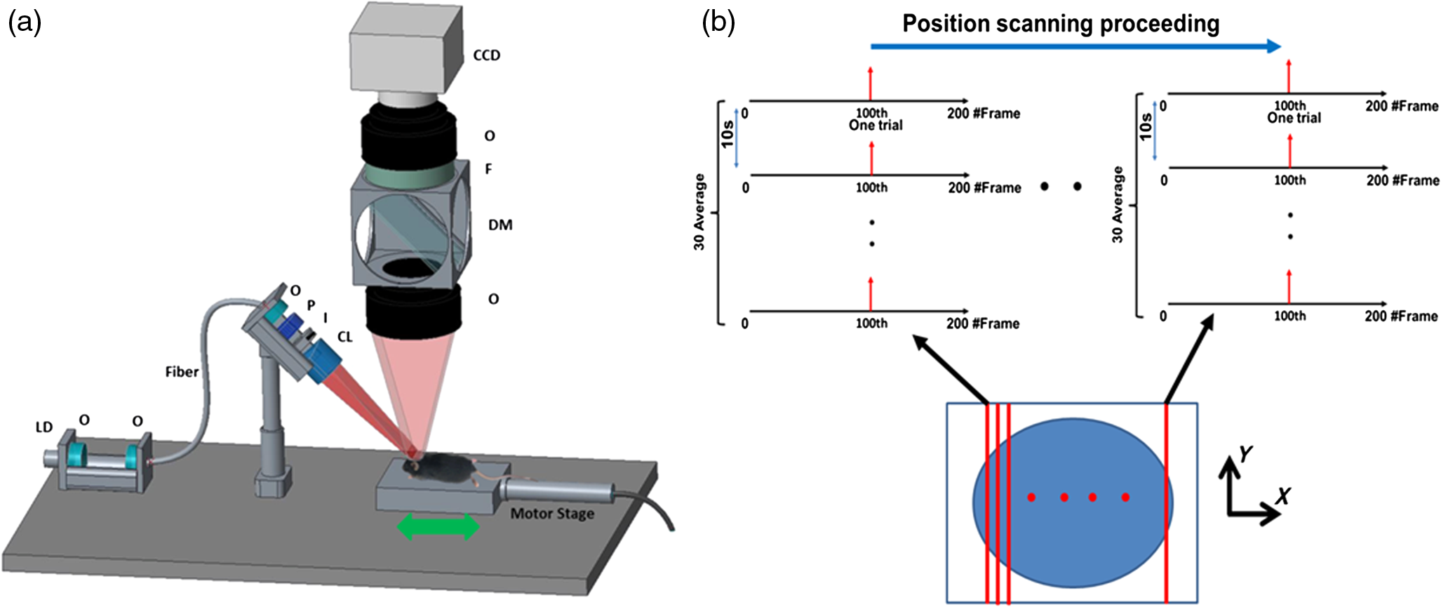
1. Introduction

Visualization of evoked and spontaneous neuronal activity in vivo is of great importance for understanding brain functions.¹^,² Localizing neural activities is a critical step in understanding the functional characteristics of neuronal interactions in the brain.²^–⁴ Due to both high spatial and temporal resolutions, optical imaging has become an important technique to investigate the neuronal and vascular responses to brain activation.⁵^–¹⁰ Based on either absorption, scattering, or fluorescence contrasts, various optical imaging methods have been demonstrated for functional brain mapping,⁴ including diffuse optical imaging (DOI),¹¹^–¹³ intrinsic optical signal (IOS) imaging,¹⁴^,¹⁵ multiphoton microscopy (MPM),¹⁶^,¹⁷ optical coherence tomography (OCT),¹⁸^–²² and photoacoustic tomography (PAT).²³ However, limited resolution (DOI), relatively low contrast (OCT), shallow penetration depth (IOS), or low data acquisition speed (MPM and PAT) have somehow limited their applications in imaging three-dimensional (3-D) neural activities, a process that needs both high temporal and spatial resolutions.²⁴

Laminar optical tomography (LOT) was initially developed to image absorption contrast for hemodynamic changes.²⁵^–²⁸ Soon after, it was rapidly adapted to fluorescent molecular imaging, applications termed either fluorescence laminar optical tomography (FLOT)³^,²⁸^,²⁹ or mesoscopic fluorescence molecular tomography (MFMT).³⁰^,³¹ Similar to diffuse optical tomography (DOT),³² LOT uses an array of photon detectors or a charge-coupled device (CCD) camera to collect photons emitted from locations at different distances away from the illumination position, enabling simultaneous detection of scattered light travelling through different depths in the tissue. LOT is sensitive to both absorption and fluorescence contrasts providing an axial resolution of $\sim 100$ to $200 μ m$ with several millimeters imaging depth.³^,²⁵^,²⁶^,³³ Recent studies demonstrated that angled illumination or detection modification (termed aFLOT) improves both resolution and depth sensitivity.³^,³⁴ Another rapid, noncontact depth-resolved imaging method called modulated imaging has also been developed for quantitative, wide-field characterization of optical absorption and scattering properties of turbid media, utilizing frequency-domain sampling and model-based analysis of the spatial modulation transfer function.³⁵^–³⁷

In this review paper, we focus on applications in neuroimaging using LOT. We first introduce the physical principles and instrumentation of LOT that enable depth-resolved imaging. Then, we review representative applications in 3-D imaging of the hemodynamic changes and neural activities in vivo.

2. Laminar Optical Tomography Principle and Instrumentation

2.1.

Laminar Optical Tomography Basic Principle

The working principle of LOT is based on light transport in tissues,³⁸ which includes three primary physical processes: scattering, absorption, and fluorescence. The relative probability of occurrence for each process depends upon the type of sample imaged and the wavelength of light used.³⁹ For in vivo brain imaging, scattering is the prevalent phenomenon. During light propagation, some of the photons will scatter out from the surface of the tissue. These photons will be captured by the detectors near the tissue surface with various separations from the light illumination/entrance position (source–detector separations). The light emerging at greater distances (i.e., larger source–detector separation) has a higher statistical probability of having travelled deeper into the tissue. By detecting the emerging light for a range of positions with different source–detector separations, it is possible to perform depth-resolved imaging of subsurface tissue structures through a proportional relationship between the source–detector separations and the average investigation depths.²⁸ Figure 1(a) shows the cross-sectional diagram of a typical LOT source–detector configuration and representative photon paths. The detection geometry used in LOT is similar to the detection geometry used in DOT. In contrast to DOT, in which source–detector separations are typically several centimeters,²⁴ LOT utilizes smaller source–detector separations (from several tens of microns to a few millimeters). As a result of this difference, information from a relatively shallow depth (millimeter or mesoscopic scale) is collected by the detectors, enabling tomographic imaging with a higher resolution compared to that of DOT.⁴⁰

Fig. 1

(a) Schematic of LOT source (S) and detector (D1 to D7) setup. (b) LOT system for depth-resolved hemodynamic imaging of rat cortex.²⁷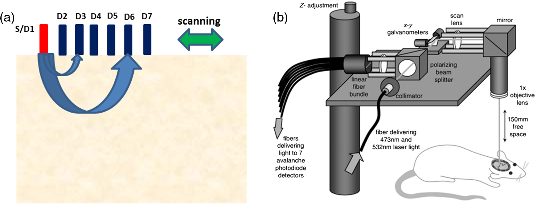

2.1.1.

Mathematical expression of laminar optical tomography based on fluorescence contrast

The linearized relationship (Born approximation) between the measured fluorescence signals $F$ and the steady-state fluorescence distribution $O$ at position $r$ can be expressed as³⁸^,⁴⁰

Eq. (1)

F (\vec{r_{n}}, \vec{r_{m}}) = \frac{1}{4 π} \int S (\vec{r} - \vec{r_{n}}) \cdot O (\vec{r}) \cdot G (\vec{r_{m}} - \vec{r}) d^{3} \vec{r} = W_{n . m} O (r),

where

Eq. (2)

O (\vec{r}) = ϵ_{ex} \cdot c (\vec{r}) \cdot γ,

where

S

is the distribution over

\vec{r}

from the excitation photon radiance in the tissue resulting from a source at position

\vec{r_{n}}

(related to the absorption and scattering coefficients, tissue anisotropy, and refractive index of the tissue at this excitation wavelength);

G

is the probability that a photon emitted by a fluorescence source at position

\vec{r}

within the tissue will be detected by the detector at

\vec{r_{m}}

(related to the absorption and scattering coefficients, tissue anisotropy, and refractive index of the tissue at this emission wavelength, respectively);

ϵ_{ex}

is the extinction coefficient of the fluorophores at the excitation wavelength;

c (\vec{r})

is the concentration of the fluorophore; and

γ

is the fluorescent quantum yield of the fluorophores. Thus, the measured fluorescence signals and the fluorescence distribution are related by

W

, which is referred to as the weight matrix or sensitivity (Jacobian) matrix and represents the likely paths (spatial sensitivity) into which the scattered photons have travelled, and also back out of the tissue. Since the fluorescence emission will always result in a longer wavelength from that of the excitation light,

W

must account for the different absorbing and scattering properties at the excitation and emission wavelengths. One common scenario for functional brain imaging is described as follows. The tissue is already fluorescent at the initial stage (e.g., loaded with voltage-sensitive dye) and then a local signal perturbation occurs (increase or decrease) in the fluorescence at a discrete region after an intended stimulation, which is similar for the absorption case. Equation (1) then can be then expressed in the following way:

Eq. (3)

Δ F (\vec{r_{n}}, \vec{r_{m}}) = \frac{1}{4 π} \int S (\vec{r} - \vec{r_{n}}) \cdot Δ O (\vec{r}) \cdot G (\vec{r_{m}} - \vec{r}) d^{3} \vec{r} = W_{n . m} Δ O (\vec{r}),

where the small signal change

Δ F

results from a small change in fluorescence distribution

Δ O

. We can imagine that when a photon interacts with a fluorophore, the photon is absorbed and a photon with a longer wavelength is emitted, which is an incoherent process so the photon loses all knowledge of its previous propagation status. So, the emission fluorescence will scatter in an isotropic way within the tissue. Furthermore, it is preferable to normalize the equation into the form known as “normalized Born.” As shown in Eq. (4), the measured fluorescence signal is normalized by

F_{0}

(the signal measured before perturbation) and the right hand side is similarly divided by

Ø_{0}

(the expected fluorescence simulated on a homogeneous medium):

Eq. (4)

\frac{Δ F}{F_{0}} = \frac{W}{Ø_{0}} Δ O .

By using “normalized Born,” it is very helpful to cancel the systematic errors related to measurements (e.g., ariations in gain between each detector).²⁴^,²⁵^,⁴¹ Also, in fluorescence LOT measurements, fluorescence signals detected from shallower layers are much stronger than those from the deeper perturbation signal. By normalizing to the original signal, it becomes possible to measure the change in fluorescence before and after the perturbation at different depths within a proper dynamic range.²⁴

2.1.2.

Mathematical expression of laminar optical tomography based on absorption contrast

For the absorption case, the detected photons scatter along a random walk path from the source to the detectors and usually the scattering is predominantly in the forward direction, so we assumed that each scattering event causes a relatively small change to the direction of the photon. The perturbed radiance can be expressed as³⁸

Eq. (5)

Δ M (\vec{r_{n}}, \vec{r_{m}}) = - \frac{1}{4 π} \int M_{0} (\vec{r} - \vec{r_{n}}) \cdot Δ μ_{a} (\vec{r}) \cdot G (\vec{r_{m}} - \vec{r}) d^{3} \vec{r} = W_{n . m} Δ μ_{a} (\vec{r}),

where

Eq. (6)

M_{0} (\vec{r_{n}}, \vec{r_{m}}) = \frac{1}{4 π} \int S (\vec{r} - \vec{r_{n}}) \cdot G (\vec{r_{m}} - \vec{r}) d^{3} \vec{r},

where

M_{0}

is the measurement of a homogeneous background,

Δ M

is the small change in measurement results from a small change in absorption

Δ μ_{a}

, while

W

in this absorption case need not account for the change of excitation and emission wavelengths. Similar to Eq. (4), the normalized form for LOT based on absorption contrast is expressed as²⁴

Eq. (7)

\frac{Δ M}{M_{0}} = \frac{W}{ϕ_{0}} Δ μ_{a},

where

M_{0}

represents the signal measured before a perturbation and

ϕ_{0}

represents the simulated signal expected from the tissue in the absence of the perturbation in absorption case.²⁴

2.2.

Forward Modeling in Laminar Optical Tomography

The spatial sensitivity matrix $W$ can be predicted using light propagation models, in which tissue scattering and absorbing properties, fluorophore characteristics (extinction coefficient and quantum yield), and the relative positions of the light source and detectors must be included. Several methods have been used to model photon propagation in scattering samples.⁴²^,⁴³ Two common types of forward modeling methods are summarized below.

2.2.1.

Radiative transfer equation based model

Time-dependent radiative transfer equation (RTE) can be used to accurately describe photon migration through tissue.⁴⁴ The diffusion approximation (DA) to the RTE is often applied since solving RTE is complex and computationally expensive, and there are analytic solutions to the infinite and semi-infinite geometry with different boundary conditions of the diffusion equation. ⁴⁵^,⁴⁶ DA has been the preferred forward model in DOT due to its computational efficiency and ease of implementation.⁴⁰^,⁴² It has been shown that DA cannot account for boundary measurements when there are structures within the scattering length from the surface of superficial tissues.⁴⁷^,⁴⁸ In other words, DA is invalid and will not provide accurate results for the small source–detector separations typically used for LOT in mesoscopic regime.

An improved DA to radiative transport, delta-P1 approximation, has been developed and validated for LOT.⁴⁹ While delta-P1 approximation can improve the computational efficiency, the estimation accuracy is moderate (with relative errors $\sim 40 %$ ). Also, there are larger relative errors when source–detector separations are very small or when the heterogeneity is very close to the source or detectors due to the intrinsic limitations of the diffusion model.⁴⁹ However, for some applications in which high speed is needed, delta-P1 approximation can be a good choice, especially for LOT based on fluorescence contrast. Furthermore, by taking advantage of the delta-isotropic phase function, the phase function corrected DA approach improves the performance of the DA and agrees with experimental results to an excellent degree, opening a potential for modeling photon propagation in LOT.⁵⁰

2.2.2.

Monte Carlo methods

By tracing the random walk steps that each photon packet takes when it travels inside the tissue, the Monte Carlo (MC) method has been used for simulating light transport in tissues for over three decades. ⁵¹^,⁵² MC provides a flexible and rigorous solution to the problem of light transport in turbid media with a complex structure.⁵³^,⁵⁴ The MC method is able to solve the RTE with a desired accuracy; hence, it is well suited to simulating the light propagation in mesoscopic regimes.⁴⁰^,⁴⁷^,⁵⁴^,⁵⁵ Compared to other analytical or empirical methods, large packets of photons need to be simulated ( $10^{5}$ to $10^{9}$ ) to obtain simulations with stochastic accuracy, requiring intensive computation and a great deal of time. A variety of methods for speeding up MC simulations, including scaling methods,⁵⁶ perturbation methods,⁵⁷ hybrid methods,⁵⁸ variation reduction techniques,⁵⁹ and parallel computation,⁶⁰^,⁶¹ has been developed.⁵⁴ The majority of LOT/MFMT work employs the MC method to compute the optical forward problem.³^,²⁷^,²⁶^,⁴⁰^,⁶²^,⁶³ Most of the current LOT/MFMT results used only homogenous forward models for generation of the spatial sensitivity $W$ , while heterogeneities (such as large blood vessels and different tissue layers) could feasibly be considered into the forward model to achieve improved fitting between the data and the model.²⁴^,⁶⁴ However, since the photon path becomes more uncertain as they scatter further, especially in complexed biological tissues, the mismatch between the mathematical model prediction and actual measurement may cause the degradation of resolution as a function of depth.³^,²⁴^,²⁸

2.3.

Image Reconstruction for Laminar Optical Tomography

After knowing $W$ , the next step is to solve Eqs. (3) or (4) to estimate the 3-D distribution of the fluorescence (or absorption) changes $Δ O (or Δ μ_{a})$ . It is challenging to solve the inverse problem since the number of measurements available is often much smaller than the number of unknown 3-D image elements (voxels), which may result in a nonunique solution.⁶⁵ Moreover, compared to transmittance geometry, solving the inverse problem for reflectance geometry is more challenging due to limited angular sampling.⁶⁶ The typical approach to solve the inverse problems is to minimize $L = W Δ O - Δ F (or L = W Δ μ_{a} - Δ M)$ using an iterative solver, with the estimate $Δ O (or Δ μ_{a})$ updated iteratively to minimize $L$ until a preset number of iterations is reached or when $L$ is below a set value (tolerance).⁴⁰ The most common iterative methods employed in the field are the conjugate gradient method,³¹ the least squares method,⁶⁷^,⁶⁸ and algebraic techniques.²⁹^,⁶⁹ However, using only these iterative solvers is still not enough since the system is ill-conditioned and very sensitive to noise propagation.⁴⁰ A regularization term is required to tolerate small mismatches between the actual measurement and the prediction using the forward model, which could result from systematic errors or noise and inaccuracies in the light propagation model.²⁴ One typical formulation of the inverse problem in LOT/MFMT is

Eq. (8)

Δ O = W^{T} {(W W^{T} + λ I)}^{- 1} Δ F [or Δ μ_{a} = W^{T} {(W W^{T} + λ I)}^{- 1} Δ M],

where

λ I

is a regularization factor, which dictates how well the data [

Δ O (or Δ μ_{a})

] fit the model [

W Δ O (or W Δ μ_{a})

].²⁴ It becomes the Tikhonov regularization if

I

is the identity matrix, which has been commonly used in LOT/MFMT. ²⁵^,³⁴ Large values of

λ

will generate superficially weighted smooth images with underestimated quantification.²⁴ Radially variant

λ I

has the potential to minimize high-frequency noise in the reconstructed image and produce constant image resolution and contrast across the image field,⁷⁰ with

I

being a diagonal matrix, whose elements are the square-root of the corresponding diagonal elements of

W^{T} W

,³²^,⁷¹ and

λ

can be selected via

L

-curve analysis.⁷²

2.4.

Laminar Optical Tomography Instrumentation

The first LOT system was reported in 2004.²⁵ Since then, several improvements or alternative designs have been investigated.³^,²⁸^,³⁰^,³¹^,⁷³^,⁷⁴ We first summarize two representative LOT systems in the following sections, and then LOT/MFMT with variant configurations and time-resolved protocol are also covered.

2.4.1.

Laminar optical tomography based on absorption contrast

In the living brain, the main absorption contrast relies on the distinctive absorption spectra of oxy- and deoxyhemoglobin ( ${HbO}_{2}$ and HbR). At visible and near-infrared wavelengths, hemoglobin in blood is the most significant absorber. Changes in blood flow, blood volume, and oxygenation can be induced following functional activities in the brain.⁷⁵ Changing the oxygenation status of blood can be inferred from the changes in the relative concentrations of ${HbO}_{2}$ and HbR. In this way, absorption properties of the brain can be related to the variations in the oxygenation state of hemoglobin and further connected to the localized neural activities. In brain research, the cortical hemodynamic response to stimulus provides a detectable signal, which can report the presence and location of neuronal activation.²⁷^,⁷⁶^,⁷⁷ Furthermore, by using different wavelengths of excitation lights and the known absorption spectra of HbR and ${HbO}_{2}$ , the changes in the concentration of ${HbO}_{2}$ and HbR can be calculated. One of the main advantages of the method based on absorption contrast is that there is no need to use any extrinsic chemical probes, which makes this approach more feasible for clinical translation. The scattering of brain tissues is often assumed not to change significantly during the hemodynamic response.⁹ While this method can record the hemodynamic responses to functional activations in the brain, the inter-relation between neural activities and hemodynamic changes is still an area of intense research.⁷⁸^–⁸³

The general schematic of a LOT system based on absorption contrast is shown in Fig. 1(b).²⁷ Illumination light from one or more lasers is first coupled into a fiber and then collimated. The collimated light then passes through a polarizing beam splitter and is steered by a pair of galvanometer scanning mirrors onto a scan lens. Together with an objective lens, the beam is focused onto the surface of the tissue. Signals collected from the tissue will pass back up through the same light path and is descanned by the galvanometers. To be able to separate the incident light and the scatter light, a strongly polarized laser is normally used. Since specular reflections from optics and the tissue surface will maintain the same polarization, light that has been scattered several times will lose its original polarization quickly. About 50% of the scattered light emerging from the sample will be successfully separated from specular reflections through the polarizing beam splitter. That successfully separated light then passes through a lens and is focused onto a linear fiber bundle or directly on the detector array.²⁷ Different from the pinhole setting in a confocal microscope, the line of fibers in the LOT system acts like seven axially offset pinholes, each leading to a separate detector corresponding to signals from different depths. As the focused beam is scanned over the surface of the tissue, scattered light emerging from the tissue at seven different depths will be collected simultaneously by the seven avalanche photodiode detectors, which results in seven two-dimensional (2-D) images per raster scan [e.g., if we choose $50 \times 50 pixels$ over a $3.5 {mm}^{2}$ field of view (FoV), then we have $50 \times 50 = 2500$ source positions and $50 \times 50 \times 7 = 17, 500$ measurements from all the detector positions.]. A faster and more sensitive second generation LOT system that utilizes three excitation wavelengths and incorporates simultaneous imaging of both absorption and fluorescence contrast has also been reported.²⁸

2.4.2.

Laminar optical tomography based on fluorescence contrast

Exogenous fluorescent dyes, as well as transgenic methods, can also provide highly specific optical contrast enhancement. They can report functional parameters, such as changes in membrane potential [voltage-sensitive dyes (VSD)] or ion concentrations (pH-, calcium-, chloride-, potassium-sensitive dyes).⁴^,⁸⁴ By binding to the neural membrane and converting changes in transmembrane voltage into the fluorescence signal of the emitted light, VSD imaging provides a useful and direct manner in revealing activities of the neural networks in the brain with relatively high spatial and temporal resolution (up to microseconds).⁴ Compared to hemodynamics imaging based on absorption contrast (slow signal changes $\sim$ second time scale), fluorescence signal change originates directly from rapid changes of neural activities, which is at the millisecond scale.⁴

The main difference of the LOT system based on fluorescence contrast compared to the LOT based on absorption contrast is the use of a dichroic mirror (for fluorescence) or a polarizing beam splitter (for absorption), and a long-pass or band-pass optical filter (depending on the type of fluorophores) before the detectors to further block the excitation light. Figure 2(a) shows one schematic diagram of a recently developed line-scanning aFLOT system.³ The excitation light from a 637-nm laser diode is collimated and then coupled into a fiber to shape the light beam. An objective lens is then used to collimate the light from the fiber and the collimated light is further expanded into line-field illumination using a cylindrical lens. The emitted fluorescent light is collected through the objective lens, dichroic mirror, emission filter, and finally focused onto a high-speed CCD camera. Since the illumination light path is not confocal with the emission light path, the dichroic mirror is optional. Both fluorescence and reflectance images can be recorded by changing the corresponding filters. This system achieves scanning by moving the sample, using a precisely controlled motor stage laterally in the scanning direction (perpendicular to the line illumination direction).³ The acquired image is in XYS format (where $X$ and $Y$ represent $X$ and $Y$ dimensions of the 2-D image acquired by CCD, $S$ represents the different scanning positions, $X = 184$ , $Y = 128$ ; $S = 120$ , with a pixel size of $\sim 23 μ m$ in the specific system introduced). To reconstruct the images, the first-order Born approximation between the measurement and the fluorophore distribution was applied on the cross-section ${FoV}_{X Z}$ , with 100 source–detector pairs and 100 scanning positions chosen to constitute 10,000 measurement modes.³ And each reconstructed ${FoV}_{X Z}$ including $100 \times 100 pixels$ with a pixel size of $\sim 23 μ m$ . Weight matrix $W$ is therefore of size $10, 000 \times 10, 000$ .³ Finally, the 3-D ${FoV}_{XYZ}$ was constituted by superimposing individual ${FoV}_{X Z}$ in the $Y$ direction (illumination line direction).³ Although a graphics processing unit was applied for parallel computation, the reconstruction process for one 3-D image still takes around 10 min. However, with parallel computation developing so rapidly, we definitely believe that the time needed for MC modeling and image reconstruction will not be a concern in the future.

Fig. 2

(a) Schematic of the aFLOT system. LD, laser diode; O, objective lens; P, polarizer; S, shutter; I, iris; CL, cylindrical lens; F, filter; DM, dichroic mirror.³ (b) Time-resolved image acquisition protocol.³

2.4.3.

Laminar optical tomography/mesoscopic fluorescence molecular tomography with variant configurations

Several LOT/MFMT systems have been reported using different source/detector and scanning configurations, including point scanning with sparse array detection,²⁶ point-scanning with dense array detection,⁶⁸ and line-scanning with dense array detection.²⁹^,³⁴ Laser diodes or solid-state lasers are typically chosen as the light source.⁴⁰ A point-focused light illumination with a one-dimensional (1-D) array detector is usually used in the LOT/MFMT system.²⁶ The 3-D images are obtained through 2-D raster scanning of the illumination point, as shown in Fig. 1(b). Alternatively, a line-field illumination with a 2-D array detector [CCD or electron multiplying CCD (EMCCD), or 2-D photomultiplier tube] can be utilized, and then only 1-D scanning is required to acquire the 3-D information, as shown in Fig. 2(a). Line-scan imaging can alleviate the complicated 2-D scanner design. While similar to confocal microscopy, the line illumination mode potentially decreases the axial resolution.⁸⁵

We should note that in LOT/MFMT, a detector closer to the illumination source will receive high light intensity, while a detector with larger source–detector separation collects a much lower signal, meaning that the detector with a larger source–detector separation may need higher gain. If possible, each detector’s gain should be chosen to match its optimal signal intensity. However, when using CCD/EMCCD as the array detector, all pixels have the same gain and exposure time, which is a main drawback of such a design and may limit the system’s dynamic range.

2.4.4.

Laminar optical tomography/mesoscopic fluorescence molecular tomography recording with time-resolved protocol

Hemodynamic response is usually slow and happens in seconds; therefore, the LOT system with $\sim 40 frames / s$ imaging speed can be utilized in studying hemodynamic responses.²⁷ In order to use LOT/MFMT to record VSD dynamics, which reflects the cellular processes at the millisecond scale,⁴ a new acquisition protocol has been investigated.³^,²⁶ Hillman et al.²⁶ first reported a time-resolved FLOT system with an effective frame rate of 667 Hz imaging speed on perfused rat hearts. Basically, it requires the biological response to be repeatable for each stimulation trial and records the time relation of the acquired data with respect to the stimulus. Recently, Tang et al.³ used aFLOT to visualize neural activities in the living animal brain using VSD. One representative image acquisition protocols for time-resolved aFLOT is illustrated in Fig. 2(b). The line-illumination light is focused on the border of the desired FoV at the beginning of recording. An experimental session including all the time related images is acquired at each scanning position (e.g., for the whisker stimulation experiment, the experimental session consists of the recording before stimulus onset, and long-enough recording after stimulus onset to cover both the activation and recovery of neuronal signals). Then, another experimental session is performed to obtain the dataset at the next illumination/collection area by moving a step in the scanning direction. This process is repeated until the entire FoV is covered. The process is similar to previously published point-scanning FLOT.²⁶ For reconstruction of data recorded using the time-resolved protocol, the measurements from multiple detectors at different scanning positions with the same frame number (or corresponding to the same time points in a dynamic process) should be first regrouped as one dataset. Then, the entire time course of 3-D neural responses can be obtained by repeating the reconstruction process for all time points.

3. Representative Applications in Neuroscience

In this section, we will review three representative examples of LOT/MFMT in vivo imaging applications in neuroscience. The first two are imaging hemodynamic responses using absorption contrast, targeting the cortex and the spinal cord, respectively. The last example is focalized on imaging the neural activities evoked in the whisker system of mice by deflection of a single whisker in vivo based on fluorescence contrast using VSDs.

3.1.

Laminar Optical Tomography for In Vivo Imaging of Hemodynamics in Cortex

The cortical hemodynamic response to stimulus can provide a detectable signal, which can indicate the presence and location of neuronal activation.²⁷^,⁷⁷ The LOT system shown in Fig. 1(b) has been used to perform depth-resolved optical imaging of hemodynamic responses to forepaw stimulation in the exposed rat cortex in vivo.²⁷ This new system utilizes multiwavelength scanning (473 and 532 nm) and acquires up to 10 3-D images per second.²⁷ Figure 3(a) shows the CCD camera image of the FoV, and the LOT FoV is identified by the dotted white square. Figure 3(b) shows the HbR, ${HbO}_{2}$ , and total hemoglobin (HbT) functional changes 0.6 s after cessation of the stimulus from the horizontal LOT slices. Different slices can sample and correspond to different depth regions (e.g., the slice at $600 μ m$ corresponds to deeper cortical layers (layers III–IV) and predominantly samples changes in the capillary bed). The advantage of LOT can be revealed more clearly in Figs. 3(c) and 3(d).²⁷ Vertical slices from the 3-D ${HbO}_{2}$ data in the $x$ – $z$ plane transecting a surface draining vein and the focal capillary region are extracted, which are labeled (i) and (ii) in (a) and (b), respectively.²⁷ Based on the distinctive differences among the dynamic behaviors of the arteriolar, capillary, and venous responses observed, LOT responses can be further segmented into regions, as shown in Fig. 3(e). Then, the distinctive functional temporal signatures associated with the hemodynamic response in different vascular compartments can be further investigated.²⁷ Rapid, full-field two-photon microscopy was also applied to validate the LOT findings and to further explore the vascular mechanisms of the hemodynamic response in vivo.²⁷

Fig. 3

LOT of the cortical hemodynamic response to forepaw stimulus in rat.²⁷ (a) CCD image of rat cortical surface through thinned skull. The region imaged using LOT is indicated by the white dotted lines. m, medial; c: caudal.²⁷ (b) Depth-resolved LOT images of oxy-, deoxy- and total hemoglobin concentration changes in the cortex 0.6 s after cessation of a 4 s forepaw stimulus at cortical depths of 0, 200, and $600 μ m$ .²⁷ (c) Depth-resolved cross-section of the ${HbO}_{2}$ response at the position indicated with (i) in panel (b), representing a large draining vein. The corresponding ${HbO}_{2}$ , HbR, and HbT depth-resolved time-courses around $x = 1800 μ m$ (dotted white line) are shown to the right.²⁷ (d) Depth-resolved cross-section of the ${HbO}_{2}$ response at the position indicated with (ii) in panel b. The corresponding ${HbO}_{2}$ , HbR, and HbT depth resolved time-courses around $x = 750 μ m$ are shown to the right. Numbers on each temporal trace represent their depth of origin in microns. “a,” “v,” and “c” denote regions identified as arteriole, vein, and capillary.²⁷ (e) Isosurface rendering of hemodynamic response resolved into arterial, capillary, and venous compartments based on their distinctive temporal behaviors (40% isosurface).²⁷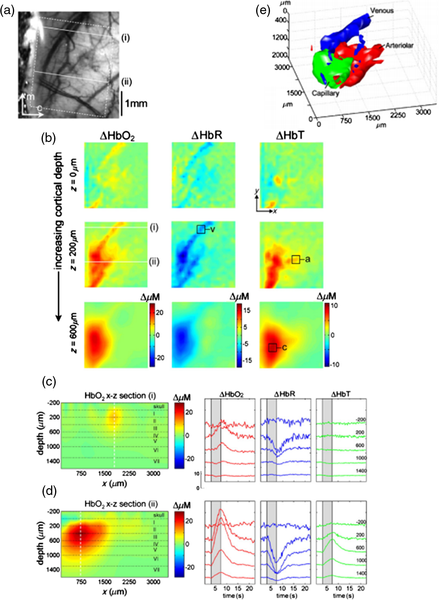

3.2.

Hemodynamics of Spinal Cord

Spinal cord trauma is a serious injury and it is crucial to understand post-traumatic neuronal reorganization in the spinal cord.⁸⁶ In a recent study, Ouakli et al.⁸⁶ investigated LOT for imaging spinal cord activation following electrode stimulation in the left hind paw, with simultaneous intrinsic optical imaging of the cortex in rats. This study indicates that LOT is a potentially powerful imaging method to study activation in the spinal cord and subsequent disruption after injury. The LOT system used in this study is similar to the system illustrated in Fig. 1(b) except only a 690-nm excitation light source was used, which means HbR was the principal chromophore providing absorption contrast.⁸⁶ Figures 4(a) and 4(b) show the simultaneously quantified activation in the cortex and spinal cord, in which Fig. 4(a) represents LOT signals from the first detector in the spinal cord at different time points after stimulation. An initial slight dip can be seen locally in the dorsal vein at 3.6 s, which may provide evidence that neurons initially use up local oxygen more quickly than it is being supplied by the gradually increased blood flow.⁹ At 10.80 s, the increase appears on the left side of the cord indicating blood is finally drained through the dorsal vein after electrode stimulation in the left hind paw. One interesting observation is that the hemodynamic response in the spinal cord is ipsilateral compared to the contralateral response in the cortex, as shown in Fig. 4(b). Figures 4(c) and 4(d) show the reconstructed images. Most response is ipsilateral on superficial layers of the dorsal horn, as shown in Fig. 4(c), which corresponds well to the location of gray matter in the spinal cord in Fig. 4(d). On the other hand, the signal in deeper sections of the spinal cord appears more diffused. Also, contralateral response is observed, which may originate from interneuron connections. Further improvements are needed to increase the imaging depth in order to image deeper signals.

Fig. 4

(a) Time course of LOT signals, induced by left hind paw stimulation, collected over 15 s at the $0.9 \times muscle threshold$ (detector 1 with a source–detector separation of $575 μ m$ ).⁸⁶ (b) Photo of the exposed cortex (left) and maximum IOS acquired simultaneously on the somatosensory cortex (right).⁸⁶ (c) 3-D map of neural activation in the spinal cord induced by left hind paw stimulation at the $0.9 \times muscle threshold$ . Ipsilateral activation around $z = 0.4 mm$ is consistent with interneuron activation.⁸⁶ (d) Reconstruction viewed across the segmented volume along the line in (c).⁸⁶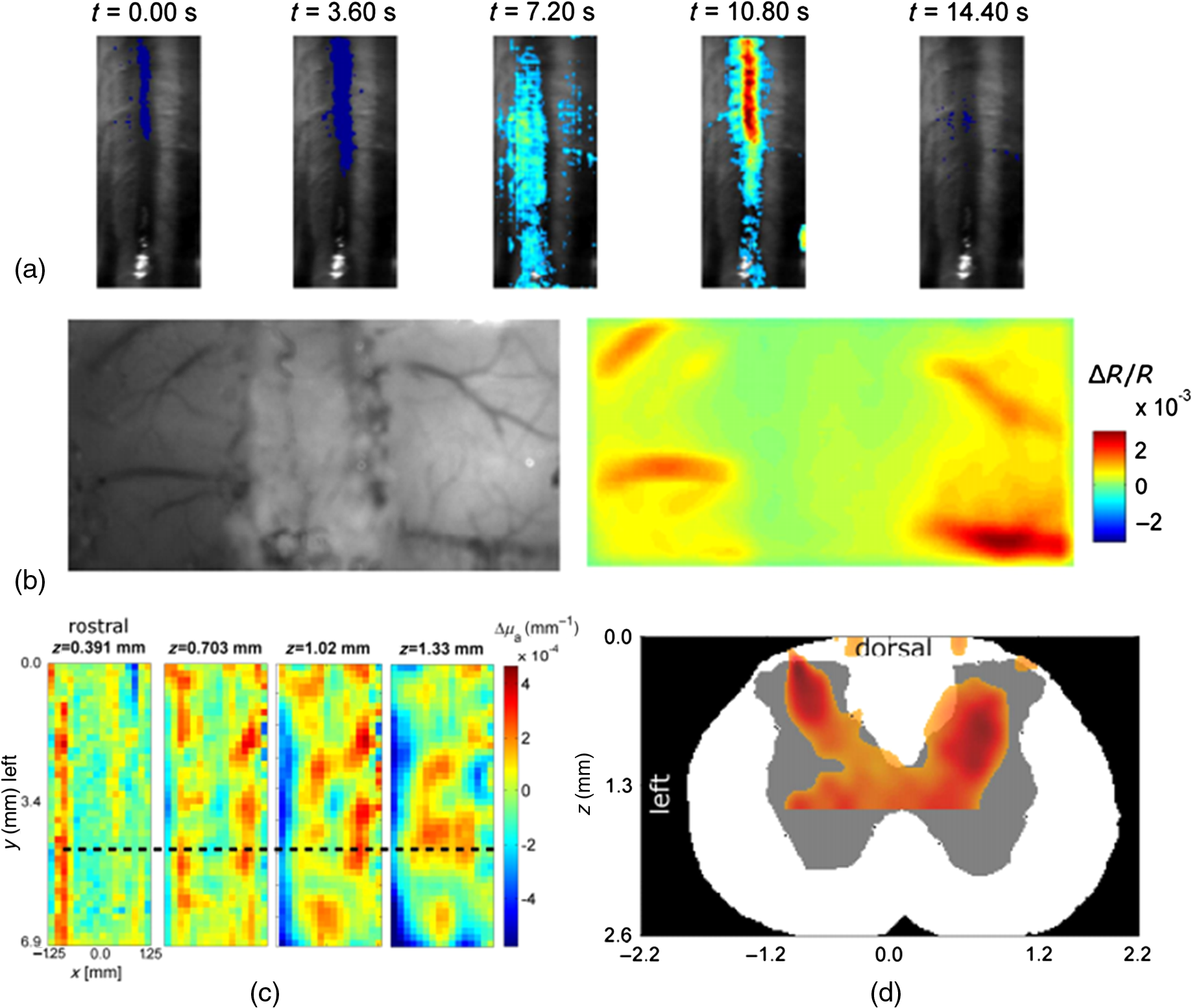

3.3.

Fluorescence Laminar Optical Tomography for Brain Cortex Imaging with Voltage-Sensitive Dyes

The rodent whisker-barrel system serves as an excellent model to investigate the development, organization, function, and plasticity of mammalian sensory pathways.⁸⁷ In this system, whiskers on the snout are represented by neuronal modules at the brainstem (barrelettes), thalamic (barreloids), and neocortical (barrels) levels.⁸⁷^–⁸⁹ The barrel fields are close to the brain surface, therefore, many imaging studies have been carried out at this region.¹⁰^,⁹⁰^–⁹⁸ However, virtually all of the previous in vivo VSD cortical imaging studies obtain only 2-D depth-integrated responses, lacking depth-dependent information. Recently, by combining aFLOT with VSDs, in vivo 3-D neural activities in the whisker barrel cortex of mice following deflection of a single whisker have been demonstrated with 5-ms temporal resolution. This study utilized the aFLOT system and time-resolved protocol, as shown in Figs. 2(a) and 2(b). In this study, system performance was first characterized by imaging a quantum-dot-embedded hydrogel and $100 - μ m$ glass capillary tube in living mouse brain. Although the accuracy and resolution of aFLOT degraded with depth, the reconstruction distortion was within $\pm 120 μ m$ up to $800 μ m$ depth (see Fig. 5), covering up to layer V in the cortex of young mice. In addition to the 3-D static system performance evaluation, a rapid response to direct electrical stimulation through the use of a bipolar electrode in the living mouse brain was observed to verify the time-resolved protocol. Then, aFLOT was used to record 3-D neural activities evoked in the barrel cortex by deflection of a single whisker in vivo. The C2 whisker was used for 20-ms mechanical stimulation, performed by an air-puff stimulator. Figure 6 shows the 3-D aFLOT reconstructed changes in fluorescence [ $Δ F / F$ (%), ordinate] following C2 whisker stimulation. The appearance of the signal was about 30 ms after the stimulus. After reaching its peak at 50 ms, the activated signals disappeared gradually. Furthermore, the results can be used to extract the 3-D dynamic activity patterns, which serve as a 3-D imaging tool to study the neural network processing in different parts of the cerebral cortex.³

Fig. 5

3-D PSFs of the aFLOT system at $302 μ m$ (a), $664 μ m$ (b), and (c) $785 μ m$ .³ Insets show the isosurface of PSFs with $μ_{s}^{'} = 0.5 / mm$ . Legends report FWHM in $μ m$ in $x$ , $y$ , and $z$ directions. (d) FWHM versus depths. Filled and open circles and multiplication symbols represent, respectively, the FWHM in $x$ , $y$ , and $z$ directions of a single PSF at the corresponding depth.³ (e,f) Reconstructed 3-D aFLOT fluorescence images of $100 - μ m$ glass capillary tube superimposed with OCT data.³

Fig. 6

3-D changes in fluorescence [ $Δ F / F$ (%), ordinate] in response to the C2 whisker stimulation reconstructed by the aFLOT system. Time period after stimulation is indicated at the bottom right corner of each image.³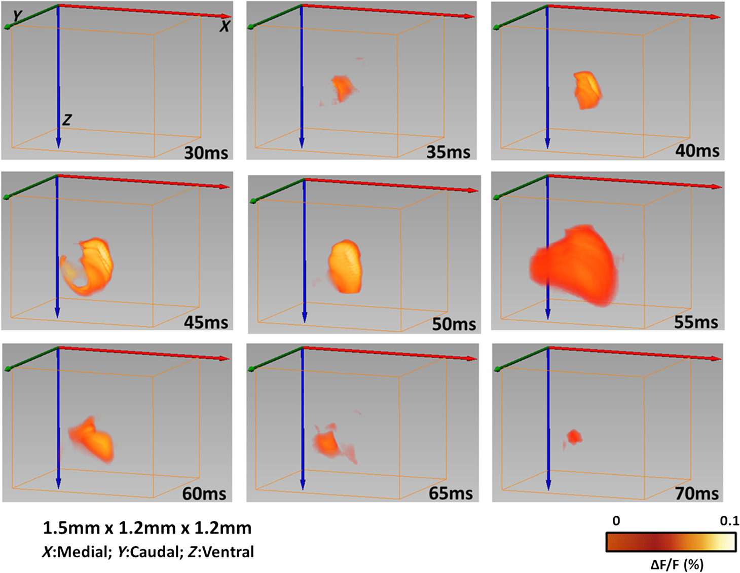

4. Summary

The 3-D imaging techniques enabling examination of spatiotemporal patterns of neuronal activities will definitely provide more details in explaining how neural networks operate in the living brain. In this paper, we first review the fundamental basis of the LOT/MFMT system, including the MC method, which is usually used to model photon propagation, and common iterative methods and regularization models for image reconstruction. Specific LOT/MFMT systems based on absorption and fluorescence are described in detail, including the data acquisition process, data size, and image reconstruction process. And, finally, three representative examples of LOT/MFMT in vivo imaging applications in neuroscience are presented.

By adopting a microscopy-based setup and DOT imaging principles, LOT/MFMT can perform 3-D imaging with higher resolution 100 to $200 μ m$ than DOT and deeper penetration (2 to 3 mm) than confocal and two-photon microscopy while there is always a trade-off between axial resolution and penetration depth. Due to the limited penetration depth of LOT/MFMT, thinning or exposing the skull is usually necessary when imaging the cortical hemodynamic responses or neural activities using LOT/MFMT, which indicates that imaging the brain with LOT/MFMT is mainly applicable in small-sized animals.³^,²⁷ In such cases, LOT/MFMT has been focused to applications in which tissues of interest are superficial, such as the exposed mouse brain and skin, as well as oncological applications.²⁴^,⁷⁴^,³⁴^,⁹⁹ For instance, LOT/MFMT has been applied to image skin cancers to describe the depth and thickness of pigmented skin lesions in clinical settings⁹⁹ and has also been employed to image the biodistribution of a photodynamic therapeutic agent with ultrasound co-registration in skin cancer models in vivo, though we can see there is still a long way to human clinical translation.⁷⁴ Imaging of internal organs using LOT/MFMT can be potentially achieved via endoscopic, intraluminal, or an intrasurgical imaging setup.²⁴ Laser scanning microscopy (e.g., confocal and two-photon microscopy) aims to reject light that has been scattered to obtain high-resolution images of the tissue either by isolating the signal from the focus using a conjugated pinhole or by employing the nonlinear effect.¹⁰⁰^,¹⁰¹ Instead, LOT/MFMT takes advantage of the scattered light so that they are much more sensitive to the optical signal changes in the tissue. LOT/MFMT obtains depth-resolved information by measuring the scattered light emerging from the tissue using detectors at different distances from the source illumination position, instead of scanning the tissue in the axial direction, which can dramatically improve the data acquisition efficiency. On the other hand, since the detected light undergoes multiple scattering in the tissue, the resolution of LOT/MFMT cannot compete with laser scanning microscopy. Moreover, estimation of photon migration using the mathematical models could not be exact, especially for the complicated biological tissues and the path of photons that become more uncertain as they scatter further. LOT/MFMT faces resolution deterioration of these reconstructed images as a function of depth.³^,²⁴^,²⁸ A combination of dense spatial datasets with regularization terms like compressive sensing-based methods has the potential to push LOT/MFMT resolution close to $100 μ m$ or beyond, even at depths of several millimeters.⁴⁰ In terms of image visualization, since laser scanning microscopy uses a more “direct” way to obtain intensity of every pixel in the image, it can achieve nearly real-time image feedback. While applying MC modeling and regularization term to solve the inverse problem, LOT/MFMT has a high computational burden and is time-consuming especially for a system with high source–detector density, as mentioned in Sec. 2.4. As a result, for now, LOT/MFMT cannot provide the reconstructed image in real time, perhaps restricting the translation to clinical applications. With the advent of the supercomputer, the time needed for high-burden computation in LOT/MFMT could be alleviated significantly.

With the advantages of overcoming the scattering limit, offering relatively high resolution, multiplexing capabilities, large FoV, and high acquisition speed, LOT provides a promising imaging technique to investigate 3-D neural activities in a minimally invasive manner in vivo. By combining absorption and fluorescence LOT into one unit, it also has the potential to study neurovascular coupling since hemodynamic responses and neural activities can be imaged by absorption and fluorescence LOT, respectively. Being able to achieve depth-resolved imaging of both absorption and fluorescence contrast, LOT/MFMT is also a promising nondestructive imaging tool in oncological applications and the tissue engineering area.

Acknowledgments

We thank Drs. Hyounguk Jang, Jianting Wang, Dmitry Lenkov, and Anna Volnova for their helpful discussions. This work is supported by NIH grants NS039050 (RSE), NS084818 (RSE), R21EB012215 (YC) and R01EB014946 (YC), NSF grant CBET-1254743 (YC), and UMB-UMCP Seed Grant (RSE and YC). The effort in completing this review paper does not involve the use of animal and/or human subjects. The results presented are cited from the published literature noted in the references. The authors declare no conflict of interest.

References

1.

A. Muto et al., “Real-time visualization of neuronal activity during perception,” Curr. Biol., 23 307 –311 (2013). http://dx.doi.org/10.1016/j.cub.2012.12.040 Google Scholar

2.

Q. Tang et al., “In vivo voltage-sensitive dye imaging of subcortical brain function,” Sci. Rep., 5 17325 (2015). http://dx.doi.org/10.1038/srep17325 Google Scholar

3.

Q. Tang et al., “In vivo mesoscopic voltage-sensitive dye imaging of brain activation,” Sci. Rep., 6 25269 (2016). http://dx.doi.org/10.1038/srep25269 Google Scholar

4.

V. Tsytsarev, C. Bernardelli and K. I. Maslov, “Living brain optical imaging: technology, methods and applications,” J. Neurosci. Neuroeng., 1 180 –192 (2012). http://dx.doi.org/10.1166/jnsne.2012.1020 Google Scholar

5.

H. S. Orbach, L. B. Cohen and A. Grinvald, “Optical mapping of electrical activity in rat somatosensory and visual cortex,” J. Neurosci., 5 1886 –1895 (1985). Google Scholar

6.

A. Grinvald et al., “Optical imaging of neuronal activity,” Physiol. Rev., 68 1285 –366 (1988). Google Scholar

7.

A. Villringer and B. Chance, “Non-invasive optical spectroscopy and imaging of human brain function,” Trends Neurosci., 20 435 –442 (1997). http://dx.doi.org/10.1016/S0166-2236(97)01132-6 Google Scholar

8.

G. Gratton and M. Fabiani, “The event-related optical signal: a new tool for studying brain function,” Int. J. Psychophysiol., 42 109 –121 (2001). http://dx.doi.org/10.1016/S0167-8760(01)00161-1 Google Scholar

9.

E. M. Hillman, “Optical brain imaging in vivo: techniques and applications from animal to man,” J. Biomed. Opt., 12 051402 (2007). http://dx.doi.org/10.1117/1.2789693 Google Scholar

10.

V. Tsytsarev et al., “Study of the cortical representation of whisker directional deflection using voltage-sensitive dye optical imaging,” Neuroimage, 53 233 –238 (2010). http://dx.doi.org/10.1016/j.neuroimage.2010.06.022 NEIMEF 1053-8119 Google Scholar

11.

F. Tian, G. Alexandrakis and H. Liu, “Optimization of probe geometry for diffuse optical brain imaging based on measurement density and distribution,” Appl. Opt., 48 2496 –504 (2009). http://dx.doi.org/10.1364/AO.48.002496 Google Scholar

12.

B. R. White and J. P. Culver, “Phase-encoded retinotopy as an evaluation of diffuse optical neuroimaging,” Neuroimage, 49 568 –577 (2010). http://dx.doi.org/10.1016/j.neuroimage.2009.07.023 NEIMEF 1053-8119 Google Scholar

13.

C. Zhou et al., “Diffuse optical monitoring of hemodynamic changes in piglet brain with closed head injury,” J. Biomed. Opt., 14 (3), 034015 (2009). http://dx.doi.org/10.1117/1.3146814 Google Scholar

14.

B. Li et al., “Altered resting-state functional connectivity after cortical spreading depression in mice,” Neuroimage, 63 1171 –1177 (2012). http://dx.doi.org/10.1016/j.neuroimage.2012.08.024 NEIMEF 1053-8119 Google Scholar

15.

A. K. Dunn et al., “Simultaneous imaging of total cerebral hemoglobin concentration, oxygenation, and blood flow during functional activation,” Opt. Lett., 28 28 –30 (2003). http://dx.doi.org/10.1364/OL.28.000028 Google Scholar

16.

A.F. McCaslin et al., “In vivo 3D morphology of astrocyte-vasculature interactions in the somatosensory cortex: implications for neurovascular coupling,” J. Cereb. Blood Flow Metab., 31 795 –806 (2011). http://dx.doi.org/10.1038/jcbfm.2010.204 Google Scholar

17.

S. Sakadzic et al., “Two-photon high-resolution measurement of partial pressure of oxygen in cerebral vasculature and tissue,” Nat. Methods, 7 755 –759 (2010). http://dx.doi.org/10.1038/nmeth.1490 Google Scholar

18.

Y. Chen et al., “Optical coherence tomography (OCT) reveals depth-resolved dynamics during functional brain activation,” J. Neurosci. Methods, 178 162 –173 (2009). http://dx.doi.org/10.1016/j.jneumeth.2008.11.026 Google Scholar

19.

V. J. Srinivasan et al., “Optical coherence microscopy for deep tissue imaging of the cerebral cortex with intrinsic contrast,” Opt. Express, 20 2220 –39 (2012). http://dx.doi.org/10.1364/OE.20.002220 Google Scholar

20.

J. Qin et al., “Fast synchronized dual-wavelength laser speckle imaging system for monitoring hemodynamic changes in a stroke mouse model,” Opt. Lett., 37 4005 –7 (2012). http://dx.doi.org/10.1364/OL.37.004005 Google Scholar

21.

H. Wang et al., “Reconstructing micrometer-scale fiber pathways in the brain: multi-contrast optical coherence tomography based tractography,” Neuroimage, 58 984 –992 (2011). http://dx.doi.org/10.1016/j.neuroimage.2011.07.005 NEIMEF 1053-8119 Google Scholar

22.

L. Yu et al., “Spectral Doppler optical coherence tomography imaging of localized ischemic stroke in a mouse model,” J. Biomed. Opt., 15 066006 (2010). http://dx.doi.org/10.1117/1.3505016 Google Scholar

23.

X. Wang et al., “Noninvasive laser-induced photoacoustic tomography for structural and functional in vivo imaging of the brain,” Nat. Biotechnol., 21 803 –806 (2003). http://dx.doi.org/10.1038/nbt839 Google Scholar

24.

E. M. C. Hillman and S. A. Burgess, “Sub-millimeter resolution 3D optical imaging of living tissue using laminar optical tomography,” Laser Photonics Rev., 3 159 –179 (2009). http://dx.doi.org/10.1002/lpor.v3:1/2 LPRAB8 1863-8880 Google Scholar

25.

E. M. C. Hillman et al., “Laminar optical tomography: demonstration of millimeter-scale depth-resolved imaging in turbid media,” Opt. Lett., 29 1650 –1652 (2004). http://dx.doi.org/10.1364/OL.29.001650 OPLEDP 0146-9592 Google Scholar

26.

E. M. Hillman et al., “Depth-resolved optical imaging of transmural electrical propagation in perfused heart,” Opt. Express, 15 17827 (2007). http://dx.doi.org/10.1364/OE.15.017827 Google Scholar

27.

E. M. C. Hillman et al., “Depth-resolved optical imaging and microscopy of vascular compartment dynamics during somatosensory stimulation,” Neuroimage, 35 89 –104 (2007). http://dx.doi.org/10.1016/j.neuroimage.2006.11.032 NEIMEF 1053-8119 Google Scholar

28.

B. Yuan et al., “A system for high-resolution depth-resolved optical imaging of fluorescence and absorption contrast,” Rev. Sci. Instrum., 80 043706 (2009). http://dx.doi.org/10.1063/1.3117204 Google Scholar

29.

S. Yuan et al., “Three-dimensional coregistered optical coherence tomography and line-scanning fluorescence laminar optical tomography,” Opt. Lett., 34 1615 –1617 (2009). http://dx.doi.org/10.1364/OL.34.001615 OPLEDP 0146-9592 Google Scholar

30.

M. S. Ozturk et al., “Mesoscopic fluorescence molecular tomography of reporter genes in bioprinted thick tissue,” J. Biomed. Opt., 18 100501 (2013). http://dx.doi.org/10.1117/1.JBO.18.10.100501 JBOPFO 1083-3668 Google Scholar

31.

L. L. Zhao et al., “The integration of 3-D cell printing and mesoscopic fluorescence molecular tomography of vascular constructs within thick hydrogel scaffolds,” Biomaterials, 33 5325 –5332 (2012). http://dx.doi.org/10.1016/j.biomaterials.2012.04.004 BIMADU 0142-9612 Google Scholar

32.

V. Venugopal and X. Intes, “Recent advances in optical mammography,” Curr. Med. Imaging Rev., 8 244 –259 (2012). http://dx.doi.org/10.2174/157340512803759884 Google Scholar

33.

Y. Chen et al., “Integrated optical coherence tomography (OCT) and fluorescence laminar optical tomography (FLOT),” IEEE J. Sel. Top. Quantum Electron., 16 755 –766 (2010). http://dx.doi.org/10.1109/JSTQE.2009.2037723 IJSQEN 1077-260X Google Scholar

34.

C. W. Chen and Y. Chen, “Optimization of design parameters for fluorescence laminar optical tomography,” J. Innovative Opt. Health Sci., 4 309 –323 (2011). http://dx.doi.org/10.1142/S1793545811001435 Google Scholar

35.

D. J. Cuccia et al., “Quantitation and mapping of tissue optical properties using modulated imaging,” J. Biomed. Opt., 14 024012 (2009). http://dx.doi.org/10.1117/1.3088140 JBOPFO 1083-3668 Google Scholar

36.

D. J. Cuccia et al., “Modulated imaging: quantitative analysis and tomography of turbid media in the spatial-frequency domain,” Opt. Lett., 30 1354 –1356 (2005). http://dx.doi.org/10.1364/OL.30.001354 OPLEDP 0146-9592 Google Scholar

37.

S. Gioux et al., “Three-dimensional surface profile intensity correction for spatially modulated imaging,” J. Biomed. Opt., 14 034045 (2009). http://dx.doi.org/10.1117/1.3156840 JBOPFO 1083-3668 Google Scholar

38.

A. Dunn and D. Boas, “Transport-based image reconstruction in turbid media with small source-detector separations,” Opt. Lett., 25 1777 –1779 (2000). http://dx.doi.org/10.1364/OL.25.001777 OPLEDP 0146-9592 Google Scholar

39.

S. L. Jacques, “Optical properties of biological tissues: a review,” Phys. Med. Biol., 58 R37 –R61 (2013). http://dx.doi.org/10.1088/0031-9155/58/11/R37 Google Scholar

40.

M. S. Ozturk et al., “Mesoscopic fluorescence molecular tomography for evaluating engineered tissues,” Ann. Biomed. Eng., 44 667 –679 (2016). http://dx.doi.org/10.1007/s10439-015-1511-4 ABMECF 0090-6964 Google Scholar

41.

E. M. C. Hillman et al., “Calibration techniques and datatype extraction for time-resolved optical tomography,” Rev. Sci. Instrum., 71 3415 –3427 (2000). http://dx.doi.org/10.1063/1.1287748 RSINAK 0034-6748 Google Scholar

42.

S. R. Arridge and J. C. Schotland, “Optical tomography: forward and inverse problems,” Inverse Prob., 25 123010 (2009). http://dx.doi.org/10.1088/0266-5611/25/12/123010 INPEEY 0266-5611 Google Scholar

43.

S. R. Arridge and M. Schweiger, “Image reconstruction in optical tomography,” Philos. Trans. R. Soc. B-Biol. Sci., 352 717 –726 (1997). http://dx.doi.org/10.1098/rstb.1997.0054 Google Scholar

44.

A. D. Klose and A. H. Hielscher, “Iterative reconstruction scheme for optical tomography based on the equation of radiative transfer,” Med. Phys., 26 1698 –1707 (1999). http://dx.doi.org/10.1118/1.598661 MPHYA6 0094-2405 Google Scholar

45.

A. Kienle and M. S. Patterson, “Improved solutions of the steady-state and the time-resolved diffusion equations for reflectance from a semi-infinite turbid medium,” J. Opt. Soc. Am. A-Opt. Image Sci. Vision, 14 246 –254 (1997). http://dx.doi.org/10.1364/JOSAA.14.000246 Google Scholar

46.

R. C. Haskell et al., “Boundary-conditions for the diffusion equation in radiative-transfer,” J. Opt. Soc. Am. A-Opt. Image Sci. Vision, 11 2727 –2741 (1994). http://dx.doi.org/10.1364/JOSAA.11.002727 Google Scholar

47.

A. K. Iranmahboob and E. M. Hillman, “Diffusion vs. Monte Carlo for image reconstruction in mesoscopic volumes,” in Biomedical Optics, (2008). Google Scholar

48.

K. M. Yoo, F. Liu and R. R. Alfano, “When does the diffusion-approximation fail to describe photon transport in random-media,” Phys. Rev. Lett., 64 2647 –2650 (1990). http://dx.doi.org/10.1103/PhysRevLett.64.2647 PRLTAO 0031-9007 Google Scholar

49.

B. Yuan, “Radiative transport in the delta-P1 approximation for laminar optical tomography,” J. Innovative Opt. Health Sci., 02 149 –163 (2009). http://dx.doi.org/10.1142/S1793545809000486 Google Scholar

50.

E. Vitkin et al., “Photon diffusion near the point-of-entry in anisotropically scattering turbid media,” Nat. Commun., 2 587 (2011). http://dx.doi.org/10.1038/ncomms1599 Google Scholar

51.

B. C. Wilson and G. Adam, “A Monte-Carlo model for the absorption and flux distributions of light in tissue,” Med. Phys., 10 824 –830 (1983). http://dx.doi.org/10.1118/1.595361 MPHYA6 0094-2405 Google Scholar

52.

L. Wang, S. L. Jacques and L. Zheng, “MCML—Monte Carlo modeling of light transport in multi-layered tissues,” Comput. Methods Programs Biomed., 47 131 –146 (1995). http://dx.doi.org/10.1016/0169-2607(95)01640-F Google Scholar

53.

D. Boas et al., “Three dimensional Monte Carlo code for photon migration through complex heterogeneous media including the adult human head,” Opt. Express, 10 159 –170 (2002). http://dx.doi.org/10.1364/OE.10.000159 OPEXFF 1094-4087 Google Scholar

54.

C. G. Zhu and Q. Liu, “Review of Monte Carlo modeling of light transport in tissues,” J. Biomed. Opt., 18 050902 (2013). http://dx.doi.org/10.1117/1.JBO.18.5.050902 JBOPFO 1083-3668 Google Scholar

55.

S. T. Flock et al., “Monte Carlo modeling of light propagation in highly scattering tissues. I. Model predictions and comparison with diffusion theory,” IEEE Trans. Biomed. Eng., 36 1162 –1168 (1989). http://dx.doi.org/10.1109/TBME.1989.1173624 IEBEAX 0018-9294 Google Scholar

56.

R. Graaff et al., “Condensed Monte Carlo simulations for the description of light transport,” Appl. Opt., 32 426 –34 (1993). http://dx.doi.org/10.1364/AO.32.000426 Google Scholar

57.

C. K. Hayakawa et al., “Perturbation Monte Carlo methods to solve inverse photon migration problems in heterogeneous tissues,” Opt. Lett., 26 1335 –1337 (2001). http://dx.doi.org/10.1364/OL.26.001335 OPLEDP 0146-9592 Google Scholar

58.

L. H. Wang and S. L. Jacques, “Hybrid model of Monte-Carlo simulation and diffusion-theory for light reflectance by turbid media,” J. Opt. Soc. Am. A-Opt. Image Sci. Vision, 10 1746 –1752 (1993). http://dx.doi.org/10.1364/JOSAA.10.001746 Google Scholar

59.

Q. Liu and N. Ramanujam, “Sequential estimation of optical properties of a two-layered epithelial tissue model from depth-resolved ultraviolet-visible diffuse reflectance spectra,” Appl. Opt., 45 4776 –4790 (2006). http://dx.doi.org/10.1364/AO.45.004776 APOPAI 0003-6935 Google Scholar

60.

E. Alerstam, T. Svensson and S. Andersson-Engels, “Parallel computing with graphics processing units for high-speed Monte Carlo simulation of photon migration,” J. Biomed. Opt., 13 060504 (2008). http://dx.doi.org/10.1117/1.3041496 JBOPFO 1083-3668 Google Scholar

61.

Q. Q. Fang and D. A. Boas, “Monte Carlo simulation of photon migration in 3D turbid media accelerated by graphics processing units,” Opt. Express, 17 20178 –20190 (2009). http://dx.doi.org/10.1364/OE.17.020178 OPEXFF 1094-4087 Google Scholar

62.

J. Chen and X. Intes, “Comparison of Monte Carlo methods for fluorescence molecular tomography-computational efficiency,” Med. Phys., 38 5788 –5798 (2011). http://dx.doi.org/10.1118/1.3641827 MPHYA6 0094-2405 Google Scholar

63.

A. R. Gardner, C. K. Hayakawa and V. Venugopalan, “Coupled forward-adjoint Monte Carlo simulation of spatial-angular light fields to determine optical sensitivity in turbid media,” J. Biomed. Opt., 19 065003 (2014). http://dx.doi.org/10.1117/1.JBO.19.6.065003 JBOPFO 1083-3668 Google Scholar

64.

E. M. Hillman et al., “Differential imaging in heterogeneous media: limitations of linearization assumptions in optical tomography,” Proc. SPIE, 4250 327 –338 (2001). http://dx.doi.org/10.1117/12.434511 PSISDG 0277-786X Google Scholar

65.

F. Yang et al., “High-resolution mesoscopic fluorescence molecular tomography based on compressive sensing,” IEEE Trans. Biomed. Eng., 62 248 –255 (2015). http://dx.doi.org/10.1109/TBME.2014.2347284 IEBEAX 0018-9294 Google Scholar

66.

B. W. Pogue et al., “Comparison of imaging geometries for diffuse optical tomography of tissue,” Opt. Express, 4 270 –286 (1999). http://dx.doi.org/10.1364/OE.4.000270 OPEXFF 1094-4087 Google Scholar

67.

W. Zhu et al., “Iterative total least-squares image reconstruction algorithm for optical tomography by the conjugate gradient method,” J. Opt. Soc. Am. A, 14 799 –807 (1997). http://dx.doi.org/10.1364/JOSAA.14.000799 Google Scholar

68.

S. Bjorn, V. Ntziachristos and R. Schulz, “Mesoscopic epifluorescence tomography: reconstruction of superficial and deep fluorescence in highly-scattering media,” Opt. Express, 18 8422 –8429 (2010). http://dx.doi.org/10.1364/OE.18.008422 OPEXFF 1094-4087 Google Scholar

69.

X. Intes et al., “Projection access order in algebraic reconstruction technique for diffuse optical tomography,” Phys. Med. Biol., 47 N1 (2002). http://dx.doi.org/10.1088/0031-9155/47/1/401 PHMBA7 0031-9155 Google Scholar

70.

B. W. Pogue et al., “Spatially variant regularization improves diffuse optical tomography,” Appl. Opt., 38 2950 –2961 (1999). http://dx.doi.org/10.1364/AO.38.002950 APOPAI 0003-6935 Google Scholar

71.

R. Endoh, M. Fujii and K. Nakayama, “Depth-adaptive regularized reconstruction for reflection diffuse optical tomography,” Opt. Rev., 15 51 –56 (2008). http://dx.doi.org/10.1007/s10043-008-0009-9 1340-6000 Google Scholar

72.

X. Intes et al., “In vivo continuous-wave optical breast imaging enhanced with indocyanine green,” Med. Phys., 30 1039 –1047 (2003). http://dx.doi.org/10.1118/1.1573791 MPHYA6 0094-2405 Google Scholar

73.

S. A. Burgess et al., “Fiber-optic and articulating arm implementations of laminar optical tomography for clinical applications,” Biomed. Opt. Express, 1 780 –790 (2010). http://dx.doi.org/10.1364/BOE.1.000780 Google Scholar

74.

M. S. Ozturk et al., “Mesoscopic fluorescence tomography of a photosensitizer (HPPH) 3D biodistribution in skin cancer,” Acad. Radiol., 21 271 –280 (2014). http://dx.doi.org/10.1016/j.acra.2013.11.009 Google Scholar

75.

R. P. Friedland and C. Iadecola, “Roy and Sherrington (1890) — a centennial reexamination of on the regulation of the blood-supply of the brain,” Neurology, 41 10 (1991). http://dx.doi.org/10.1212/WNL.41.1.10 NEURAI 0028-3878 Google Scholar

76.

P. T. Fox and M. E. Raichle, “Focal physiological uncoupling of cerebral blood-flow and oxidative-metabolism during somatosensory stimulation in human-subjects,” Proc. Natl. Acad. Sci. U. S. A., 83 1140 –1144 (1986). http://dx.doi.org/10.1073/pnas.83.4.1140 Google Scholar

77.

T. A. Woolsey et al., “Neuronal units linked to microvascular modules in cerebral cortex: Response elements for imaging the brain,” Cereb. Cortex, 6 647 –660 (1996). http://dx.doi.org/10.1093/cercor/6.5.647 Google Scholar

78.

N. Li et al., “Study of the spatial correlation between neuronal activity and BOLD fMRI responses evoked by sensory and channelrhodopsin-2 stimulation in the rat somatosensory cortex,” J. Mol. Neurosci., 53 553 –561 (2014). http://dx.doi.org/10.1007/s12031-013-0221-3 JMNEES 0895-8696 Google Scholar

79.

A. L. Vazquez et al., “Neural and hemodynamic responses elicited by forelimb- and photo-stimulation in channelrhodopsin-2 mice: insights into the hemodynamic point spread function,” Cereb. Cortex, 24 2908 –2919 (2014). http://dx.doi.org/10.1093/cercor/bht147 Google Scholar

80.

B. Iordanova et al., “Neural and hemodynamic responses to optogenetic and sensory stimulation in the rat somatosensory cortex,” J. Cereb. Blood Flow Metab., 35 922 –932 (2015). http://dx.doi.org/10.1038/jcbfm.2015.10 Google Scholar

81.

A. S. Salinet et al., “A systematic review of cerebral hemodynamic responses to neural activation following stroke,” J. Neurol., 260 2715 –2721 (2013). http://dx.doi.org/10.1007/s00415-013-6836-z Google Scholar

82.

A. Devor et al., “Coupling of total hemoglobin concentration, oxygenation, and neural activity in rat somatosensory cortex,” Neuron, 39 353 –359 (2003). http://dx.doi.org/10.1016/S0896-6273(03)00403-3 NERNET 0896-6273 Google Scholar

83.

S. A. Sheth et al., “Linear and nonlinear relationships between neuronal activity, oxygen metabolism, and hemodynamic responses,” Neuron, 42 347 –355 (2004). http://dx.doi.org/10.1016/S0896-6273(04)00221-1 NERNET 0896-6273 Google Scholar

84.

M. I. Kotlikoff, “Genetically encoded Ca²⁺ indicators: using genetics and molecular design to understand complex physiology,” J. Physiol., 578 55 –67 (2007). http://dx.doi.org/10.1113/jphysiol.2006.120212 Google Scholar

85.

A. A. Tanbakuchi, A. R. Rouse and A. F. Gmitro, “Monte Carlo characterization of parallelized fluorescence confocal systems imaging in turbid media,” J. Biomed. Opt., 14 044024 (2009). http://dx.doi.org/10.1117/1.3194131 JBOPFO 1083-3668 Google Scholar

86.

N. Ouakli et al., “Laminar optical tomography of the hemodynamic response in the lumbar spinal cord of rats,” Opt. Express, 18 10068 –10077 (2010). http://dx.doi.org/10.1364/OE.18.010068 OPEXFF 1094-4087 Google Scholar

87.

R. S. Erzurumlu, Y. Murakami and F. M. Rijli, “Mapping the face in the somatosensory brainstem,” Nat. Rev. Neurosci., 11 252 –263 (2010). http://dx.doi.org/10.1038/nrn2804 Google Scholar

88.

I. Vitali and D. Jabaudon, “Synaptic biology of barrel cortex circuit assembly,” Semin. Cell Dev. Biol., 35 156 –164 (2014). http://dx.doi.org/10.1016/j.semcdb.2014.07.009 Google Scholar

89.

R. S. Erzurumlu and P. Gaspar, “Development and critical period plasticity of the barrel cortex,” Eur. J. Neurosci., 35 1540 –1553 (2012). http://dx.doi.org/10.1111/ejn.2012.35.issue-10 Google Scholar

90.

C.H. Chen-Bee et al., “Whisker array functional representation in rat barrel cortex: transcendence of one-to-one topography and its underlying mechanism,” Front Neural Circuits, 6 93 (2012). http://dx.doi.org/10.3389/fncir.2012.00093 Google Scholar

91.

B. R. Lustig et al., “Voltage-sensitive dye imaging reveals shifting spatiotemporal spread of whisker-induced activity in rat barrel cortex,” J. Neurophysiol., 109 2382 –2392 (2013). http://dx.doi.org/10.1152/jn.00430.2012 Google Scholar

92.

B. F. Grewe et al., “High-speed in vivo calcium imaging reveals neuronal network activity with near-millisecond precision,” Nat. Methods, 7 399 –405 (2010). http://dx.doi.org/10.1038/nmeth.1453 Google Scholar

93.

C. C. Petersen, “The functional organization of the barrel cortex,” Neuron, 56 339 –355 (2007). http://dx.doi.org/10.1016/j.neuron.2007.09.017 NERNET 0896-6273 Google Scholar

94.

T. Y. Mao et al., “Long-range neuronal circuits underlying the interaction between sensory and motor cortex,” Neuron, 72 111 –123 (2011). http://dx.doi.org/10.1016/j.neuron.2011.07.029 NERNET 0896-6273 Google Scholar

95.

I. Petrof, A. N. Viaene and S. M. Sherman, “Properties of the primary somatosensory cortex projection to the primary motor cortex in the mouse,” J. Neurophysiol., 113 2400 –2407 (2015). http://dx.doi.org/10.1152/jn.00949.2014 JONEA4 0022-3077 Google Scholar

96.

N. Weiler et al., “Top-down laminar organization of the excitatory network in motor cortex,” Nat. Neurosci., 11 360 –366 (2008). http://dx.doi.org/10.1038/nn2049 NANEFN 1097-6256 Google Scholar

97.

C. C. H. Petersen, “Cortical control of whisker movement,” Ann. Rev. Neurosci., 37 183 –203 (2014). http://dx.doi.org/10.1146/annurev-neuro-062012-170344 Google Scholar

98.

D. Feldmeyer et al., “Barrel cortex function,” Prog. Neurobiol., 103 3 –27 (2013). http://dx.doi.org/10.1016/j.pneurobio.2012.11.002 PGNBA5 0301-0082 Google Scholar

99.

T. J. Muldoon et al., “Analysis of skin lesions using laminar optical tomography,” Biomed. Opt. Express, 3 1701 –1712 (2012). http://dx.doi.org/10.1364/BOE.3.001701 BOEICL 2156-7085 Google Scholar

100.

A. Boyde, “Stereoscopic images in confocal (tandem scanning) microscopy,” Science, 230 1270 –1272 (1985). http://dx.doi.org/10.1126/science.4071051 SCIEAS 0036-8075 Google Scholar

101.

W. Denk, J. H. Strickler and W. W. Webb, “Two-photon laser scanning fluorescence microscopy,” Science, 248 73 –76 (1990). http://dx.doi.org/10.1126/science.2321027 SCIEAS 0036-8075 Google Scholar

Biography

Qinggong Tang received his BS degree in optoelectronics from Huazhong University of Science and Technology, Wuhan, China, in 2012. He is currently a PhD candidate in the Fischell Department of Bioengineering at the University of Maryland, College Park. His interests include biophotonics and imaging, optical coherence tomography, multiphoton microscopy, fluorescence laminar optical tomography and their applications in neuroscience, and cancer research.

Jonathan Lin is an undergraduate student working toward his BS degree in bioengineering at the University of Maryland, College Park, and will graduate in the spring of 2017. He currently works as a research assistant at the Biophotonics Lab there and is the CEO and cofounder of Reflective Information, Inc., a startup company that develops smart devices with advanced image processing software.

Vassiliy Tsytsarev has a PhD in neuroscience from Saint-Petersburg State University in Russia. Soon after graduation, he moved to Japan and started work in the Brain Science Institute of RIKEN and Kyoto University. After 7 years in Japan, he moved to the United States and is now working at the University of Maryland. Functional brain mapping, neural circuits, and different types of brain optical imaging are his main scientific interests, as well as professional background.

Reha S. Erzurumlu is a professor of anatomy and neurobiology at the University of Maryland, School of Medicine. He received his PhD from the University of California Irvine and did postdoctoral work at Brown University and M.I.T. He is an established investigator with expertise in development, plasticity, and organization of sensory systems. His research uses the rodent trigeminal system as a model and employs numerous approaches ranging from molecular biology, tissue culture, immunohistochemistry, morphology, electrophysiology, imaging, and behavior.

Yi Liu received his BS degree in optoelectronics from Huazhong University of Science and Technology, Wuhan, China, in 2015. Now, he is a PhD student at the Fischell Department of Bioengineering at the University of Maryland, College Park. His scientific interests include bioimaging, optical diagnostic devices, fluorescence laminar optical tomography, and redox fluorescence imaging.

Yu Chen is currently an associate professor and associate chair of the Fischell Department of Bioengineering, University of Maryland, College Park. His research interests include optical coherence tomography, laminar optical tomography, multiphoton microscopy, development of quantitative optical sensing and imaging devices for clinical translation, and preclinical and clinical applications of optical technologies in imaging brain function, renal physiology, cancer therapy, and tissue engineering.

Citation Download Citation

Qinggong Tang, Jonathan Lin, Vassiliy Tsytsarev, Reha S. Erzurumlu, Yi Liu, and Yu Chen "Review of mesoscopic optical tomography for depth-resolved imaging of hemodynamic changes and neural activities," Neurophotonics 4(1), 011009 (14 November 2016). https://doi.org/10.1117/1.NPh.4.1.011009

Published: 14 November 2016

Access the abstract

JOURNAL ARTICLE
12 PAGES

DOWNLOAD PAPER SAVE TO MY LIBRARY

GET CITATION

CITATIONS

Cited by 18 scholarly publications.

Explore citations on Lens.org

RIGHTS & PERMISSIONS

Get copyright permission Get copyright permission on Copyright Marketplace

KEYWORDS

Luminescence

Sensors

Optical tomography

Absorption

Imaging systems

Hemodynamics

Tissue optics

1.

Introduction

2.

Laminar Optical Tomography Principle and Instrumentation

2.1.

Laminar Optical Tomography Basic Principle

Fig. 1

2.1.1.

Mathematical expression of laminar optical tomography based on fluorescence contrast

Eq. (1)

Eq. (2)

Eq. (3)

Eq. (4)

2.1.2.

Mathematical expression of laminar optical tomography based on absorption contrast

Eq. (5)

Eq. (6)

Eq. (7)

2.2.

Forward Modeling in Laminar Optical Tomography

2.2.1.

Radiative transfer equation based model

2.2.2.

Monte Carlo methods

2.3.

Image Reconstruction for Laminar Optical Tomography

Eq. (8)

2.4.

Laminar Optical Tomography Instrumentation

2.4.1.

Laminar optical tomography based on absorption contrast

2.4.2.

Laminar optical tomography based on fluorescence contrast

Fig. 2

2.4.3.

Laminar optical tomography/mesoscopic fluorescence molecular tomography with variant configurations

2.4.4.

Laminar optical tomography/mesoscopic fluorescence molecular tomography recording with time-resolved protocol

3.

Representative Applications in Neuroscience

3.1.

Laminar Optical Tomography for In Vivo Imaging of Hemodynamics in Cortex

Fig. 3

3.2.

Hemodynamics of Spinal Cord

Fig. 4

3.3.

Fluorescence Laminar Optical Tomography for Brain Cortex Imaging with Voltage-Sensitive Dyes

Fig. 5

Fig. 6

4.

Summary

Acknowledgments

References

Biography

Show All Keywords

Keywords/Phrases

Search In:

Publication Years