|
|
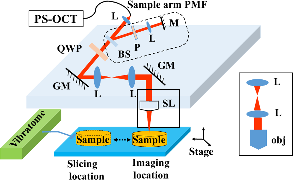
1.IntroductionIn addition to coordination of movement, studies show that the cerebellum participates in other brain activities including certain cognitive function and experience-dependent adaptive process.1–3 Even though the cerebrum occupies the predominant volume in the brain, the cerebellum holds the majority of brain neurons across different species of mammals.4,5 The neurons in the cerebellum are mainly located in the tightly folded cerebellar cortex, which can be further divided into, from outside to inside, molecular, Purkinje cell, and granular layers. Abundant nerve fiber tracts connect the cerebellum with other brain regions through cerebellar peduncles. Diseases involving the cerebellum often lead to motor disturbance and loss of movement coordination.6 Optical coherence tomography (OCT) produces depth resolved images (cross sections) of tissue structures at the micrometer scale resolution.7 In recent years, OCT for brain imaging has drawn attention because of the increasing research interest in brain microstructure and circuitry. In addition to the visualizations of cortical layers and neurons,8–11 OCT has been used to study pathological changes in brain conditions such as brain tumors,12–14 edema,15 and seizures.16 OCT has also been shown to separate different layers in the cerebellar cortex17,18 and Purkinje cell bodies13 in the cerebellum. Reflectivity, the conventional contrast for OCT and confocal microscopy, may not be descriptive enough to delineate different structures in complex tissue. Polarization-sensitive OCT (PS-OCT)19 provides additional contrasts that originate from tissue birefringence. It distinguishes white matter and gray matter, and visualizes nerve fiber tracts in the brain.20 PS-OCT highlights the myelinated and birefringent nerve fibers with the retardance contrast and indicates the in-plane fiber alignment with the axis orientation contrast. To facilitate large-scale imaging at microscopic resolution, a tissue slicer has been integrated with PS-OCT to form the serial optical coherence scanner (SOCS).21 Brain imaging with SOCS showed that the reflectivity contrast portrays morphology, and the polarization contrasts primarily probe myelinated nerve fibers in the white matter. Architecture of nerve fibers delineated by retardance and the in-plane fiber orientations quantified by optic axis orientation have been covalidated with diffusion MRI.22 In this study, we used SOCS to visualize and map the cerebellum and nearby brainstem areas of ex vivo mouse brains. Reflectivity- and polarization-based intrinsic contrasts are utilized for coronal or sagittal sections. Stacking several sections allows reconstruction of a large three-dimensional (3-D) volume, in which the global anatomy is visualized and the nerve fiber pathways are tracked. By incorporating a water immersion objective, we also present higher resolution tiled images that delineate fine structures in the coronal and sagittal planes. The movements of stage for imaging or slicing steps are computer controlled, and the entire process is semiautomated. The results show that SOCS is an efficient tool to image rodent cerebellum at microscopic resolution and it offers a viable technique for studying cerebellar diseases. 2.Methods2.1.Sample PreparationAdult C57BL/6J wide type mice were euthanized and transcardially perfused by 10% buffered formalin. All animal treatments and experiments are in accordance with the Institutional Animal Care and Use Committee at the University of Minnesota approved protocols. Dissected brains were kept in 10% buffered formalin for 48 h prior to imaging. Only the cerebellum and adjacent brain stem region were scanned by SOCS. Samples were imaged in coronal and sagittal sections. After imaging the superficial region of a sample, a slice was removed by the vibratome slicer to access the next section. 2.2.Optical SetupSOCS21 integrates polarization maintaining fiber (PMF)-based spectral domain PS-OCT23 and a vibratome tissue slice. To obtain absolute optic axis orientation, calibration is included for dynamic removal of a phase offset.24 The light source is a 25-mW superluminescent diode with 840-nm center wavelength and 50-nm FWHM bandwidth, yielding an axial resolution of in tissue (refractive index: ). Linearly polarized light is coupled into one of the PMF channels in a fiber bench and split into reference and sample arms by a PMF coupler. Briefly, light in the reference arm (not shown) passes through a quarter-wave plate (QWP) whose optic axis is 22.5 deg with respect to the incoming polarization state. As a result, light returning from a reflector passes through the QWP one more time and becomes linearly polarized at 45 deg. This ensures equal powers propagating in the orthogonal channels of PMF toward the coupler, where interference of light returning from the reference and sample arms occurs. Details of the optical setup including the spectrometer design, operation, and performance can be found in Ref. 23. Figure 1 shows the sample arm configuration. Linearly polarized light emerging from PMF is collimated by a lens (). Light passes through a beam sampler, which diverts a small portion of the beam toward the calibration unit (dashed box) consisting of a polarizer and a mirror. After passing a QWP with optic axis set at 45 deg with respect to the incoming linear state, light becomes circularly polarized. Galvanometer controlled scanning mirrors provide beam scanning in two lateral dimensions. A beam expander () consisting of two achromatic lenses is positioned between the scanning mirrors to pivot the light at the back focal plane of a scan lens or a microscope objective and to increase the effective numerical aperture. This system is capable of imaging samples using two different schemes. Solid boxes in Fig. 1 show switchable parts for selecting either a scan lens (LSM03-BB , Thorlabs, Inc., Newton, New Jersey) or a water immersion objective (UMPLFLN W, Olympus, Co., Tokyo, Japan) with another beam expander, respectively. For the latter, the required space can be gained by removing the vibratome or by raising the height of the main platform. The FWHM lateral resolution is with the scan lens or with the objective. Imaging with high NA microscope objectives relates to optical coherence microcopy that can also utilize polarization sensitivity for high-resolution brain imaging.25 In our setup, the optical path of the reference arm is also adjustable to accommodate the path length change due to switching between the scan lens and the objective. Light reflected/backscattered within a birefringent sample can be represented by an elliptical polarization state that results in variable light powers coupled back into the PMF channels. In the coupler, light from the reference and sample arms interfere in the corresponding PMF channels. 2.3.Contrasts and Image FormationSpectra from two orthogonal polarization channels are focused side-by-side onto a single line-scan camera in a custom spectrometer. Acquired spectra are resampled in linear -space. Dispersion compensation is performed in software.26 Inverse Fourier transform of interference-related spectral oscillations yields complex depth profiles that are in the form of , where and denote the amplitude and phase as a function of depth and the subscripts represent the polarization channels.27 Reflectivity, , phase retardance, , and relative axis orientation, information of the depth profile (A-line), are obtained by and where is an arbitrary offset due to PMF and it is potentially time-varying with fiber movement and temperature change. is measured from the interference of the calibration paths (the path in reference arm is not shown), which is positioned below the imaging area dedicated to the tissue sample. Absolute optic axis orientation is computed by subtracting the offset from the orientation measurement, .24 Correspondingly, the in-plane orientation of white matter tracts is determined by dynamic calibration.A cross-sectional image is formed by stacking several A-lines acquired during a lateral scan (-axis). Multiple cross sections are acquired during raster scan to construct a 3-D volume. En-face images are two-dimensional (2-D) projections of the 3-D datasets onto the -plane. The en-face images can be generated from different contrasts in a number of ways. For example, the en-face reflectivity image can get its pixel values from the average reflectivity values within the depth profiles. It is useful to present the anatomical structures in 2-D for the imaged section. Likewise, the en-face retardance images are produced by averaging to delineate the nerve fiber tracts. A median filter is applied to the cross-sectional image prior to averaging in -direction. For the en-face orientation image, absolute optic axis orientation values within each A-line are binned into 5 deg intervals, and the mean value of Gaussian fitted histogram determines the pixel value. Axis orientation values are color coded in Hue-saturation-value (HSV) space as illustrated by a color wheel, while the brightness of colors is regulated by the en-face retardance values that highlight the white matter regions. Light intensity in tissue decays exponentially due to scattering and absorption events. Since cross-sectional reflectivity images are typically presented in logarithmic scale, the attenuation corresponds to a linear decay for uniform samples. Therefore, the values in an en-face attenuation image are calculated by a least-square first-order polynomial fitting of the logarithmic reflectivity signal within the depth profiles. The en-face birefringence image is produced by taking least-square first-order polynomial fitting of the retardance signal, as the derivative of measured retardance yields the apparent birefringence. Depth range used in calculations matches the physical slice thickness. Open source image processing tool Fiji was used to produce composite images and stitch tiles for high-resolution imaging.28 Anatomical identifications are carefully compared with Allen mouse brain atlas.29,30 Abbreviations of anatomical structures also match with Allen mouse brain atlas. 2.4.Serial imagingSerial imaging is semiautomated. A custom program written in LabView (National Instruments, Austin, Texas) controls linear actuators (T-NA series, Zaber Technologies Inc., Vancouver, British Columbia, Canada) of a one-inch three-axis translation stage, which accomplishes the repositioning of the sample. The actuators have maximum speed, repeatability and backlash. As shown in Fig. 1, separate positions for imaging and slicing could be a requirement to avoid the slicer blade interfering with the sample arm optics. The vibratome is manually controlled. The workflow of the imaging/slicing procedure is described as follows.
The optical imaging for a single-volumetric scan takes 25 s when 500 cross sections each with 1000 A-lines are acquired with an A-line rate of 20 kHz. However, the imaging and slicing procedure for a section took 4 min due to a low speed of the vibratome blade to maintain slicing quality. The raster scans covered for coronal sections and for sagittal sections. Consequently, the A-line spacing was and for coronal and sagittal cross sections, respectively. Spacing between the cross sections was , which is close to the beam diameter in the field of focus that the scan lens provides. After completing SOCS imaging for an entire sample, the scan lens and the vibratome were removed. Then, the water-immersion microscope objective as shown in Fig. 1 was incorporated for imaging selected slices at high lateral resolution. A raster scan in this case covered an area of . In order to cover the entire lateral plane, several locations with 5% overlapping region had to be scanned. Each scan included 500 cross sections, each of which contained 500 A-lines. The computer controlled the procedure with the software moving the actuators between the optical scans. High-resolution smaller-scale images are then stitched together to create a tiled image of the tissue section. 3.Results3.1.Differentiation of Anatomy from Cross-Sectional ImagesFigure 2 shows cross-sectional reflectivity and retardance images containing the cerebellum, the fourth ventricle (V4), and the brainstem, and compares the contrasts in anatomical regions. The scan for the reflectivity [Fig. 2(a)] and retardance [Fig. 2(d)] images was taken from the midline region of a coronal section which is at about Bregma as compared with the stereotaxic coordinates of the mouse brain.31 Scale bars in Fig. 2(a) represent 1 mm in -axis and 0.1 mm in -axis. A color-coded bar is shown to label different anatomy. Molecular layer (ML, blue), granular layer (GL, green), and white matter (WM, red) regions are indicated by color-coded boxes above the images. The thin Purkinje cell layer is not visualized in these cross-sectional images. Comparisons in the subplots also share the same color-coding for these anatomical structures. Fig. 2Differentiation of white matter and cerebellar cortical layers. (a) Reflectivity and (d) retardance images show a cross section of cerebellum and brainstem. The color-coded bars above the images indicate different anatomical regions (blue: ML, green: GL, red: white matter). For each region, reflectivity and phase retardance profiles of twenty A-lines are averaged and the results are plotted in (b) and (e) with the same color-coding. The slopes of reflectivity (attenuation) and retardance (birefringence) are calculated by line-fitting. The slopes are also calculated for each A-line, and the mean and standard deviations are presented in (c) and (f) with statistical significance. Scale bars in (a): -axis, 1 mm; -axis, 0.1 mm. 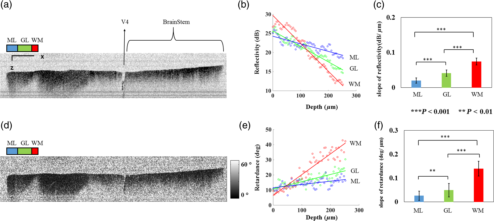 We calculated and compared the attenuation of the OCT signal in cerebellar ML, GL, and WM. Twenty A-lines were chosen from each of these regions, and the reflectivity signals in dB scale were averaged and fitted with a least-square first-order polynomial function. Figure 2(b) shows the averages (dots) and fitted lines as a function of depth. The attenuations of the OCT signal in the ML, GL, and WM region are found to be , , and , respectively. Clearly, light in the white matter region decayed faster than the layers. Attenuation for each A-line was also calculated. Figure 2(c) shows the mean and standard deviation of these attenuations in the aforementioned regions. Unpaired two-sample student -tests were performed for every pair of the three regions. Attenuations in the cerebellar ML, GL, and WM are all significantly different from each other (). This suggests that the attenuation map can be useful for delineating the two cerebellar cortex layers, and at the same time differentiating the white matter from the gray matter. We performed a similar comparison with the retardance contrast, which is represented as phase retardance [Eq. (2)]. Figure 2(e) shows the averaged retardance values as a function of depth. Averages were calculated for each region using the same twenty A-lines chosen earlier. Figure 2(e) also shows the slopes of retardance (apparent birefringence) by line fitting. The white matter region clearly exhibits the largest birefringence in the group. Calculated from each A-line, the apparent birefringence values are given in Fig. 2(f) as , , and for the ML, GL, and WM regions, respectively. Statistical comparison demonstrates the slope of retardance for the WM is significantly different from two cerebellar cortex layers (). The slopes of two cerebellar cortex layers were also significantly different from each other but with a lower -value (). The difference between the attenuation and birefringence values in GL and ML can be attributed to the anatomy of the cerebellar cortex, as GL is densely packed with small granule cells and contains myelinated axons. WM is composed of bundles of myelinated axons, and therefore, the optical properties of myelin is associated with the results. 3.2.Visualizations with En-Face Coronal ImagesFigure 3 shows en-face images of a coronal section. Comparing the images with the stereotaxic coordinates of the mouse brain,31 the section is located at about Bregma . Images are derived from the reflectivity, retardance, and axis-orientation contrasts as described in Sec. 2.3. Figure 3(a) shows the en-face reflectivity image that shows the gross anatomy. The GL can be distinguished from the ML and white matter tracts. The scale bar represents 1 mm and the labels of anatomical structures are given only in this image. Figure 3(b) shows the en-face retardance image that highlights the white matter connections in the section. Figure 3(c) shows a composite image with the green and red channels representing the reflectivity [Fig. 3(a)] and retardance [Fig. 3(b)] images, respectively. Figures 3(d) and 3(e) show the attenuation and apparent birefringence maps. Figure 3(f) shows the en-face axis orientation image with orientation values given in the color wheel. The axis orientations of the branches of arbor viate (arb) agree with the anatomical geometry. Fig. 3En-face images of a coronal section by SOCS: (a) reflectivity, (b) retardance, (d) attenuation, (e) birefringence, and (f) optic axis orientation. The composite image with reflectivity (green) and retardance (red) is in (c). The axis orientation in (f) is presented with HSV colors (see the color wheel for orientations), and the brightness is regulated by retardance values. Abbreviations: arbor viate (arb), medial longitudinal fascicle (mlf), interior cerebellar peduncle, (icp) and spinal tract of the trigeminal nerve (sptV). Scale bar: 1 mm. 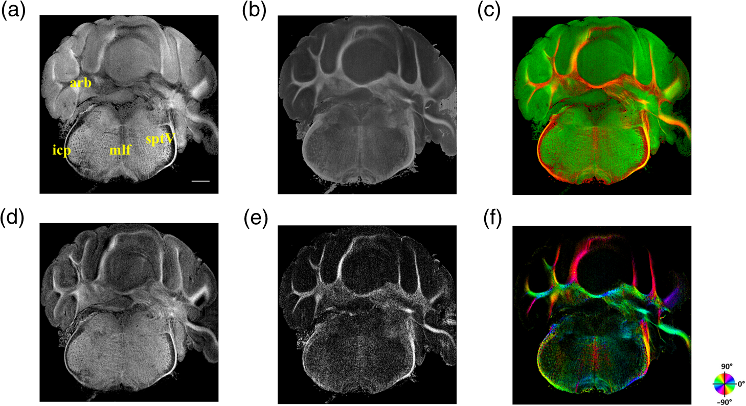 The medial longitudinal fascicle (mlf) in the midline of medulla is visualized in Figs. 3(a), 3(b), and 3(f). The inner interior cerebellar peduncle (icp), and the outer spinal tract of the trigeminal nerve (sptV) are adjacent to each other in medulla. However, in the coronal section, the inclination angle of sptV is higher than icp. Measured reflectivity, retardance [Figs. 3(a) and 3(b)], and their slopes [Figs. 3(d) and 3(e)] for the sptV are lower than the ones for the icp region. The high inclination angle of the sptV also reduces the apparent birefringence and makes the axis orientation measurement unreliable. By replacing the scan lens with the water immersion microscope objective, fine structures in the cerebellum and brainstem are delineated at high resolution. The coronal section, previously imaged with the scan lens (Fig. 3) and removed by the slicer, was positioned under the objective. Figure 4 shows the tiled image consisting of smaller-scale high-resolution images and two selected regions to highlight structures with different contrasts. The composite image in Fig. 4(a) is created by merging the en-face reflectivity (green) and retardance (red) images. Anatomical structures are presented in remarkable details. Two regions of interest (ROI) enclosed by white dashed lines are further investigated. Figures 4(b)–4(d) show fine structures in ROI-1 with the en-face reflectivity, retardance, and optic axis orientation images. In Fig. 4(b), three layers in cerebellar cortex are clearly visualized with the Purkinje cell layer (arrow) appearing as an interface between GL and ML. Compared to the arb region, the cerebellar nuclei (CBN) region has less white matter and consequently appears with reduced reflectivity and retardance. Medulla oblongata in ROI-2 [Figs. 4(e)–4(g)] consists of abundant nuclei. Reflectivity contrast [Fig. 4(e)] shows a lattice pattern. The optical contrasts show the characteristics of icp and sptV [labeled in Fig. 4(e)] in the high-resolution images. Fig. 4High-resolution en-face images of a coronal section. (a) Composite image of reflectivity (green) and retardance (red). Dashed boxes represent ROIs. (b) and (e) Reflectivity, (c) and (f) retardance, and (d) and (g) axis orientation images show these contrasts for the fine structures in ROI-1 and ROI-2, respectively. Arrow in (b) indicates Purkinje cell layer. Abbreviations: cerebellar nuclei (CBN), interior cerebellar peduncle (icp), and spinal tract of the trigeminal nerve (sptV). (d) and (g) Axis orientation is color coded in HSV space by the color wheel, and the brightness is regulated by retardance values. Scale bars in (a) and (b): 1 mm. 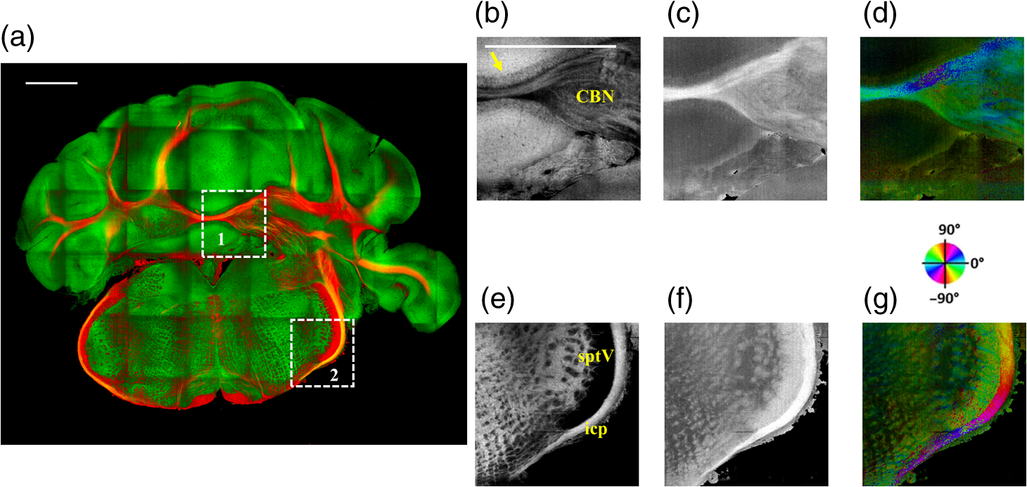 3.3.Visualizations with En-Face Sagittal ImagesTwenty sagittal sections were imaged serially with the scan lens. The sagittal section representing the en-face plane starts at lateral in the left hemisphere, and reaches lateral 1 mm across the midline into the right hemisphere. A portion of the scan (10%, or 100 A-lines in -direction) was removed from the images as it covered agarose gel supporting the tissue during slicing. As a result, the en-face images represent an area of . The en-face images were stacked together to present the anatomy in the cerebellum and brainstem. The effective volume covered with the scans is in -directions. Video 1 presents the composite en-face images of reflectivity (green) and retardance (red). Video 2, on the other hand, shows the fiber axis in the plane with the axis orientation images. Each frame in the videos represents a thick section. Scale bar is 1 mm in the videos and in Fig. 5, which shows two representative sections. Fig. 5SOCS images of two reprehensive sagittal sections. Composite images in (a) and (c) are with reflectivity (green) and retardance (red) contrasts. Axis orientation images in (b) and (d) are with colors in HSV space (see the color wheel) and the brightness of pixels is regulated by retardance values. Abbreviations: spinal trigeminal nucleus (SPN), facial nerve (vIIn). Scale bar: 1 mm. See Video 1 and Video 2 that present twenty sagittal sections with the composite and axis orientation images, respectively. Scale bars: 1 mm. (Video 1, MOV, 1.92 MB [URL: http://dx.doi.org/10.1117/1.NPh.4.1.011006.1]; Video 2, MOV, 2.54 MB [URL: http://dx.doi.org/10.1117/1.NPh.4.1.011006.2]) 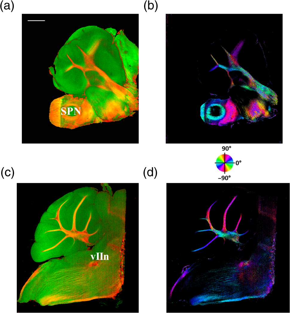 The sections shown in Fig. 5 are located at the left hemisphere at lateral [Figs. 5(a) and 5(b)] and lateral [Figs. 5(c) and 5(d)] from the midline. and lateral from the midline, respectively. Arrangement and axis orientation of the branching arb tracts are visualized in the cerebellum. Plentiful nerve tracts in the brainstem are observed since the retardance contrast highlights these connections. The spinal trigeminal nucleus [SPN in Fig. 5(a)] demonstrates lower retardance. In contrast, the surrounding fiber tracts (mainly vestibulocochlear nerve and sptV) appear red due to high birefringence. The facial nerve (vIIn) is clearly visualized in Fig. 5(c) and its position changes from interior to anterior in the videos. In Figs. 5(c) and 5(d), the sptV fibers run along the rostral edge of medulla oblongata. Several major fiber tracts such as middle cerebellar peduncle and pyramid in corticospinal tract, align with the ventral edge of medulla. Figures 5(b) and 5(d) show the in-plane axis orientations of the tracts. After imaging the entire sample, the scan lens was replaced by a water-immersion microscope objective for high-resolution imaging of one of the sagittal section presented in Figs. 5(c) and 5(d). Figure 6 shows the tiled image and two ROIs for showing the details. Figure 6(a) is the composite image of reflectivity and retardance contrasts. ROI-1 [Figs. 6(b)–6(d)] demonstrates the tightly folded cerebellar cortex and several arb tracts with the en-face reflectivity, retardance, and axis orientation images. All three layers in the cerebellar cortex are clearly presented in Fig. 6(b). The arrow indicates the darker Purkinje cell layer [Fig. 6(b)]. ROI-2 [Fig. 6(e)–6(g)] visualizes the fiber tracts in the brainstem. Retardance image [Fig. 6(f)] captures vIIn, which is located between the pons and medulla, even though the high inclination angle reduces the reflectivity and retardance contrasts. Fig. 6High-resolution en-face images of a sagittal section. (a) Composite image of reflectivity (green) and retardance (red). Dashed boxes represent ROIs. (b) and (e) Reflectivity, (c) and (f) retardance, and (d) and (g) axis orientation images show these contrasts for the fine structures in ROI-1 and ROI-2, respectively. Arrow in (b) indicates Purkinje cell layer. vIIn in (e) denotes the facial nerve. (d) and (g) Axis orientation is color coded in HSV space by the color wheel, and the brightness is regulated by retardance values. Scale bars in (a) and (b): 1 mm. 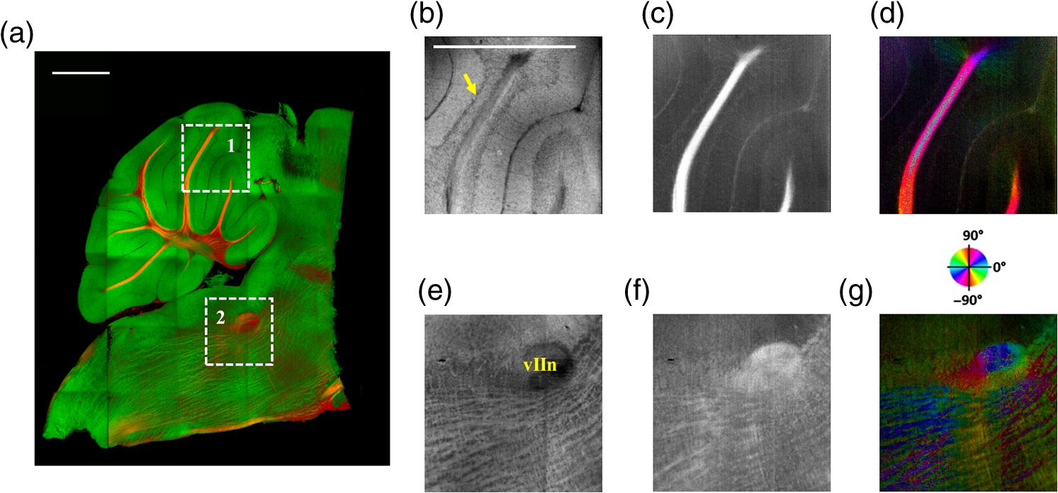 4.DiscussionVolumetric large-scale optical brain imaging at high resolution is challenging due to light scattering and limited field of view of focal lens. Recent techniques for mouse brain imaging include micro-optical sectioning tomography,32 two photon tomography,33,34 light sheet microscopy,35,36 and SOCS.21 Among these, SOCS is a label-free imaging technique and it is suitable for ex vivo imaging of the entire brain. One of the limitations is the depth of view, which may be improved to millimeter scale by using a light source operating in the longer wavelength region11 or by incorporating a tissue clearing method. The latter may reduce the contrasts. Enhancement in imaging depth could reduce the number of physical sections required for reconstructing the entire brain. The other limitation is the slicer speed to maintain good slicing quality. The system we report here is semiautomated and it only requires the user to press buttons to realize tissue slicing and data acquisition. Additional time can be saved with a fully automated system that controls the vibratome functions electronically. The current system is sufficient for a rodent brain. Imaging larger brains like primate brains is feasible, but it would require a bigger blade and longer-range stages and actuators. We can incorporate microscope objectives into SOCS to enhance lateral resolution; however, reduction in the field of view requires tile scans to cover the entire sample. The short working distance under the objective may necessitate adjustments and modifications on the stages. Moreover, the tight focus reduces the confocal parameter. Its effect for 3-D reconstruction of the sample could be avoided by shifting the focus for consecutive imaging or reducing the physical slice thickness that would increase the recording time. Quantification of attenuation would also be challenging with the microscope objective since the rapidly changing beam profile needs to be decoupled from the measurement and the focal plane may be hard to define accurately in the images. Compared with sptV in sagittal sections, the sptV fibers in coronal sections may have misinterperlation in reflectivity, retardance, and axis orientation contrasts due to high inclination angle. Related to this, the axis orientation measurement in this study is defined in a plane () orthogonal to the direction of light propagation (). However, the description of nerve fiber axis orientation in 3-D requires both azimuthal and polar angles. Computational methods37 and experimental methods utilizing measurements with variable incident angle38,24 have been proposed to retrieve 3-D axis using PS-OCT. Quantification of the fiber inclination would allow calculation of the true birefringence , since the measured apparent birefringence can be written as ,39 where is the inclination angle. Combining the information from variable incident angles after registering the 3-D datasets has potential to improve the image quality and representation of tissue anisotropy. 5.ConclusionSOCS provides an efficient approach to visualize and map the mouse cerebellum and nearby brainstem. The cerebellar layers, abundant nuclei in brainstem, and nerve fiber tracts are presented for coronal and sagittal sections at two different resolutions. Several contrasts within the anatomical structures are quantified and used in the visualizations. SOCS has the potential to study the diseases of the cerebellum and brainstem including ataxia and medulloblastoma and opens new perspectives to better understand the anatomy and pathology. AcknowledgmentsThis work was supported by research grants from the US National Science Foundation (No. NSF, CBET-1510674) and the Bob Allison Ataxia Research Center (BAARC) at the University of Minnesota. The authors would like to thank Orion Rainwater for helping with tissue preparation, and Minnesota Supercomputing Institute for the high-performance computing resources. ReferencesW. T. Thach,
“On the specific role of the cerebellum in motor learning and cognition: clues from PET activation and lesion studies in man,”
Behav. Brain Sci., 19 411
–433
(1996). http://dx.doi.org/10.1017/S0140525X00081504 BBSCDH 0140-525X Google Scholar
C. Hansel, D. J. Linden and E. D’Angelo,
“Beyond parallel fiber LTD: the diversity of synaptic and non-synaptic plasticity in the cerebellum,”
Nat. Neurosci., 4 467
–475
(2001). http://dx.doi.org/10.1038/87419 NANEFN 1097-6256 Google Scholar
R. Apps and M. Garwicz,
“Anatomical and physiological foundations of cerebellar information processing,”
Nat. Rev. Neurosci., 6
(4), 297
–311
(2005). http://dx.doi.org/10.1038/nrn1646 Google Scholar
S. Herculano-houzel, B. Mota and R. Lent,
“Cellular scaling rules for rodent brains,”
Proc. Natl. Acad. Sci., 103
(32), 12138
–12143
(2006). http://dx.doi.org/10.1073/pnas.0604911103 Google Scholar
S. Herculano-houzel and C. C. Sherwood,
“Coordinated scaling of cortical and cerebellar numbers of neurons,”
Front. Neuroanat., 4 1
–8
(2010). http://dx.doi.org/10.3389/fnana.2010.00012 Google Scholar
J. D. Schmahmann,
“Disorders of the cerebellum: ataxia, dysmetria of thought, and the cerebellar cognitive affective syndrome,”
J. Neuropsychiatry Clin. Neurosci., 16
(3), 367
–378
(2004). http://dx.doi.org/10.1176/jnp.16.3.367 Google Scholar
D. Huang et al.,
“Optical coherence tomography,”
Science, 254
(5035), 1178
–1181
(1991). http://dx.doi.org/10.1126/science.1957169 SCIEAS 0036-8075 Google Scholar
V. J. Srinivasan et al.,
“Optical coherence microscopy for deep tissue imaging of the cerebral cortex with intrinsic contrast,”
Opt. Express, 20
(3), 2220
(2012). http://dx.doi.org/10.1364/OE.20.002220 Google Scholar
C. Magnain et al.,
“Blockface histology with optical coherence tomography: a comparison with Nissl staining,”
NeuroImage, 84 524
–533
(2014). http://dx.doi.org/10.1016/j.neuroimage.2013.08.072 NEIMEF 1053-8119 Google Scholar
C. Magnain et al.,
“Optical coherence tomography visualizes neurons in human entorhinal cortex,”
Neurophoton, 2
(1), 015004
(2015). http://dx.doi.org/10.1117/1.NPh.2.1.015004 Google Scholar
S. P. Chong et al.,
“Noninvasive, in vivo imaging of subcortical mouse brain regions with optical coherence tomography,”
Opt. Lett., 40
(21), 4911
–4914
(2015). http://dx.doi.org/10.1364/OL.40.004911 OPLEDP 0146-9592 Google Scholar
H. J. Böhringer et al.,
“Imaging of human brain tumor tissue by near-infrared laser coherence tomography,”
Acta Neurochir, 151 507
–517
(2009). http://dx.doi.org/10.1007/s00701-009-0248-y Google Scholar
O. Assayag et al.,
“Imaging of non-tumorous and tumorous human brain tissues with full-field optical coherence tomography,”
NeuroImage Clin., 2 549
–557
(2013). http://dx.doi.org/10.1016/j.nicl.2013.04.005 Google Scholar
H. J. Böhringer et al.,
“Time-domain and spectral-domain optical coherence tomography in the analysis of brain tumor tissue,”
Lasers Surg. Med., 38 588
–597
(2006). http://dx.doi.org/10.1002/(ISSN)1096-9101 LSMEDI 0196-8092 Google Scholar
C. Rodriguez et al.,
“Decreased light attenuation in cerebral cortex during cerebral edema detected using optical coherence tomography,”
Neurophoton, 1 025004
(2014). http://dx.doi.org/10.1117/1.NPh.1.2.025004 Google Scholar
M. M. Eberle et al.,
“Localization of cortical tissue optical changes during seizure activity in vivo with optical coherence tomography,”
Biomed. Opt. Express, 6
(15), 1812
–1827
(2015). http://dx.doi.org/10.1364/BOE.6.001812 BOEICL 2156-7085 Google Scholar
M. E. Brezinski et al.,
“Optical biopsy with optical coherence tomography: feasibility for surgical diagnostics,”
J. Surg. Res., 71
(1), 32
–40
(1997). http://dx.doi.org/10.1006/jsre.1996.4993 Google Scholar
B. Vuong et al.,
“Measuring the optical characteristics of medulloblastoma with optical coherence tomography,”
Biomed. Opt. Express, 6
(4), 1487
(2015). http://dx.doi.org/10.1364/BOE.6.001487 Google Scholar
J. F. de Boer et al.,
“Two-dimensional birefringence imaging in biological tissue by polarization-sensitive optical coherence tomography,”
Opt. Lett., 22
(12), 934
–936
(1997). http://dx.doi.org/10.1364/OL.22.000934 OPLEDP 0146-9592 Google Scholar
H. Wang et al.,
“Reconstructing micrometer-scale fiber pathways in the brain: multi-contrast optical coherence tomography based tractography,”
NeuroImage, 58
(4), 984
–992
(2011). http://dx.doi.org/10.1016/j.neuroimage.2011.07.005 NEIMEF 1053-8119 Google Scholar
H. Wang, J. Zhu and T. Akkin,
“Serial optical coherence scanner for large-scale brain imaging at microscopic resolution,”
NeuroImage, 84 1007
–1017
(2014). http://dx.doi.org/10.1016/j.neuroimage.2013.09.063 NEIMEF 1053-8119 Google Scholar
H. Wang et al.,
“Cross-validation of serial optical coherence scanning and diffusion tensor imaging: a study on neural fiber maps in human medulla oblongata,”
NeuroImage, 100 395
–404
(2014). http://dx.doi.org/10.1016/j.neuroimage.2014.06.032 NEIMEF 1053-8119 Google Scholar
H. Wang, M. K. Al-Qaisi and T. Akkin,
“Polarization-maintaining fiber based polarization-sensitive optical coherence tomography in spectral domain,”
Opt. Lett., 35
(2), 154
–156
(2010). http://dx.doi.org/10.1364/OL.35.000154 Google Scholar
C. J. Liu et al.,
“Quantifying three-dimensional optic axis using polarization-sensitive optical coherence tomography,”
J. Biomed. Opt., 21
(7), 070501
(2016). http://dx.doi.org/10.1117/1.JBO.21.7.070501 JBOPFO 1083-3668 Google Scholar
H. Wang et al.,
“Polarization sensitive optical coherence microscopy for brain imaging,”
Opt. Lett., 41
(10), 2213
–2216
(2016). http://dx.doi.org/10.1364/OL.41.002213 Google Scholar
B. Cense et al.,
“Ultrahigh-resolution high-speed retinal imaging using spectral-domain optical coherence tomography,”
Opt. Express, 12 2435
–2447
(2004). http://dx.doi.org/10.1364/OPEX.12.002435 OPEXFF 1094-4087 Google Scholar
E. Götzinger, M. Pircher and C. K. Hitzenberger,
“High speed spectral domain polarization sensitive optical coherence tomography of the human retina,”
Opt. Express, 13
(25), 10217
–10229
(2005). http://dx.doi.org/10.1364/OPEX.13.010217 OPEXFF 1094-4087 Google Scholar
J. Schindelin et al.,
“Fiji: an open-source platform for biological-image analysis,”
Nat. Methods, 9
(7), 676
–682
(2012). http://dx.doi.org/10.1038/nmeth.2019 1548-7091 Google Scholar
E. S. Lein et al.,
“Genome-wide atlas of gene expression in the adult mouse brain,”
Nature, 445 168
–176
(2007). http://dx.doi.org/10.1038/nature05453 Google Scholar
Allen Institute for Brain Science, “Allen mouse brain atlas internet,”
(2016) http://mouse.brain-map.org June ). 2016). Google Scholar
G. Paxinos and K. Franklin, The Mouse Brain in Stereotaxic Coordinates, 4th edAcademic Press, Massachusetts
(2013). Google Scholar
A. Li et al.,
“Micro-optical sectioning tomography to obtain a high resolution atlas of the whole mouse brain,”
Science, 330
(6009), 1404
–1408
(2010). http://dx.doi.org/10.1126/science.1191776 SCIEAS 0036-8075 Google Scholar
T. Ragan et al.,
“Serial two-photon tomography for automated ex vivo mouse brain imaging,”
Nat. Methods, 9 255
–258
(2012). http://dx.doi.org/10.1038/nmeth.1854 1548-7091 Google Scholar
S. W. Oh et al.,
“A mesoscale connectome of the mouse brain,”
Nature, 508
(7495), 207
–214
(2014). http://dx.doi.org/10.1038/nature13186 Google Scholar
H. U. Dobt et al.,
“Ultramicroscopy: three-dimensional visualization of neuronal networks in the whole mouse brain,”
Nat. Methods, 4 331
–336
(2007). http://dx.doi.org/10.1038/nmeth1036 1548-7091 Google Scholar
M. B. Bouchard et al.,
“Swept confocally-aligned planar excitation (SCAPE) microscopy for high-speed volumetric imaging of behaving organisms,”
Nat. Photonics, 9 113
–119
(2015). http://dx.doi.org/10.1038/nphoton.2014.323 NPAHBY 1749-4885 Google Scholar
H. Wang, C. Lenglet and T. Akkin,
“Structure tensor analysis of serial optical coherence scanner images for mapping fiber orientations and tractography in the brain,”
J. Biomed. Opt., 20
(3), 036003
(2015). http://dx.doi.org/10.1117/1.JBO.20.3.036003 JBOPFO 1083-3668 Google Scholar
N. Ugryumova, S. V. Gangnus and S. J. Matcher,
“Three-dimensional optic axis determination using variable-incidence-angle polarization-optical coherence tomography,”
Opt. Lett., 31
(15), 2305
–2307
(2006). http://dx.doi.org/10.1364/OL.31.002305 OPLEDP 0146-9592 Google Scholar
L. Larsen et al.,
“Polarized light imaging of white matter architecture,”
Microsc. Res. Tech., 70
(10), 851
–863
(2007). http://dx.doi.org/10.1002/(ISSN)1097-0029 MRTEEO 1059-910X Google Scholar
BiographyChao J. Liu received his BS degree in optoelectronics engineering from the Huazhong University of Science and Technology, China, in 2010. He is a PhD candidate in biomedical engineering at the University of Minnesota. He is interested in quantitative optical imaging for biomedical and neuroscience applications. Kristen E. Williams received her BS degree from the University of Minnesota in biomedical engineering in 2016. After graduating, she began working for Boston Scientific Corporation as a manufacturing engineer. Her interests involve process development and process improvements for polymer extrusion. Harry T. Orr received his PhD from Washington University and completed postdoctoral fellowship at Harvard University. He is the Tulloch Professor and Director in the Institute of Translational Neuroscience at the University of Minnesota. With Huda Zoghbi, Baylor College of Medicine, he cloned spinocerebellar ataxia type 1 (SCA1) affected gene, showing CAG expansion causes SCA1. Using transgenic SCA1 mice, the group enhanced understanding pathogenesis. He is a Javits awardee (NINDS/NIH), and elected to the National Academy of Medicine in 2014. Taner Akkin received his BSc and MSc degrees in electrical and electronics engineering from Çukurova University, Turkey, in 1995 and 1997, and his PhD from the University of Texas at Austin in 2003. After postdoctoral studies at Harvard Medical School/Wellman Center for Photomedicine, Massachusetts General Hospital, he joined the Department of Biomedical Engineering at the University of Minnesota (2005), where he is an associate professor. He develops optical imaging systems to study neural structure and function. |