Correction of motion artifacts and serial correlations for real-time functional near-infrared spectroscopy

Jeffrey W. Barker; Andrea L. Rosso; Patrick J. Sparto; Theodore J. Huppert

doi:10.1117/1.NPh.3.3.031410

23 May 2016 Correction of motion artifacts and serial correlations for real-time functional near-infrared spectroscopy

Jeffrey W. Barker, Andrea L. Rosso, Patrick J. Sparto, Theodore J. Huppert

Author Affiliations +

Neurophotonics, Vol. 3, Issue 3, 031410 (May 2016). https://doi.org/10.1117/1.NPh.3.3.031410

Abstract

Functional near-infrared spectroscopy (fNIRS) is a relatively low-cost, portable, noninvasive neuroimaging technique for measuring task-evoked hemodynamic changes in the brain. Because fNIRS can be applied to a wide range of populations, such as children or infants, and under a variety of study conditions, including those involving physical movement, gait, or balance, fNIRS data are often confounded by motion artifacts. Furthermore, the high sampling rate of fNIRS leads to high temporal autocorrelation due to systemic physiology. These two factors can reduce the sensitivity and specificity of detecting hemodynamic changes. In a previous work, we showed that these factors could be mitigated by autoregressive-based prewhitening followed by the application of an iterative reweighted least squares algorithm offline. This current work extends these same ideas to real-time analysis of brain signals by modifying the linear Kalman filter, resulting in an algorithm for online estimation that is robust to systemic physiology and motion artifacts. We evaluated the performance of the proposed method via simulations of evoked hemodynamics that were added to experimental resting-state data, which provided realistic fNIRS noise. Last, we applied the method post hoc to data from a standing balance task. Overall, the new method showed good agreement with the analogous offline algorithm, in which both methods outperformed ordinary least squares methods.

1. Introduction

Near-infrared spectroscopy (NIRS) is a noninvasive technique that can monitor changes in optical absorption due to cerebral blood to detect evoked brain activity.¹ Measurements are made by an array of light sources and detectors that are coupled to the scalp through fiber optics, in a head cap worn by the subject, that are connected to the NIRS instrument. Spatially overlapping measurements that are made at multiple wavelengths within the optical window (650 to 900 nm) can allow for spectroscopic estimation of both oxyhemoglobin ( ${HbO}_{2}$ ) and deoxyhemoglobin (Hb) via the modified Beer–Lambert law.²

During a task, regional changes in blood flow and oxygen consumption in the brain alter hemoglobin levels, causing changes in the optical absorption measured by the light source to detector pairs that traverse this brain region. The nature of these evoked changes in NIRS have been shown to be related to the blood oxygen level dependent (BOLD) signal of functional magnetic resonance imaging (fMRI).³ Compared to fMRI, functional NIRS (fNIRS) offers lower spatial resolution but can be recorded at a much higher temporal resolution ( $> 10 Hz$ ). This characteristic makes fNIRS suitable for studying the temporal characteristics of the hemodynamic signal. Furthermore, fNIRS is nonrestraining, making it suitable for infants and small children and for various tasks, such as walking,⁴^,⁵ balance,⁶^–⁸ and social interaction,⁹ where fMRI is not practical.

Due to the portability and high sample rate of fNIRS measurements, several researchers have previously explored the use of fNIRS in real-time assessments of brain activity,¹⁰^–¹⁷ biofeedback,¹⁸ and brain–computer interfacing applications.¹⁵^,¹⁶^,¹⁹^–²⁴ These real-time applications, however, must contend with noise and artifacts often contained within the NIRS data. In particular, the two major sources of confounding noise that affect the analysis and interpretation of fNIRS signals are serially correlated errors due to systemic physiology, such as cardiac, respiratory, and low-frequency Mayer waves (related to blood pressure regulation), and motion artifacts due to the movement or slippage of the head cap. While several approaches to offline correction of motion²⁵^–²⁸ and physiological noise²⁹^–³¹ have been proposed, for real-time imaging, these corrections must be both automated and quickly implemented to keep up with the high sample rates of fNIRS systems. In addition, real-time correction methods need to be forward directed, meaning that they need to offer corrections using only past history data points. In contrast, many of the motion correction methods, such as wavelet or spline interpolation models,²⁶^,²⁸ use data information from both before and after the artifact for correction and thus only offer retrospective corrections.

Kalman estimation³² is an iterative method, which uses an underlying Markov process to make updates in the estimation of an underlying state (e.g., brain activity) based on a weighting of the past history of state estimates and the currently measured data. In this way, a Kalman estimator reports an estimate of the state (brain) for every sample point based on the data collected up to that point. Since the Kalman estimator algorithm is fast and forward directed, this approach has previously been used in real-time brain imaging.¹⁴

In this study, we extended the ideas of Barker et al.²⁷ to develop a real-time adaptive algorithm based on the linear Kalman filter, which allows estimation of brain activity using similar autoregressive (AR)-based prewhitening and robust regression concepts. AR prewhitening is a method to reduce the influence of structured noise such as errors due to slow drift or physiology, which have specific frequency content (termed colored noise) and are therefore not statistically random. Likewise, robust regression is a mathematical method to reduce the effect of statistical outliers, which involves an iterative process of model estimation and detection of data samples which are statistical outliers. As demonstrated by Barker et al.,²⁷ physiological noise in fNIRS data results in serially correlated noise, which violates the assumptions of an uncorrelated, independent identically distributed model error in the fit of a general linear model (GLM). If uncorrected, these nonspherical errors can result in an inaccurate control of type I error (false positives) and reduced performance of the GLM estimator. In addition, fNIRS errors often exhibit heteroscedasticity due to motion artifacts. Heteroscedasticity refers to noise that does not arise from a single uniform distribution. In the case of fNIRS, motion artifacts often have very different statistical properties (e.g., higher variance) compared to other background fluctuations. Motion artifacts often appear as statistical outliers since these errors are often much larger but less frequent and randomly occurring (nonergodic) compared to other sources of noise in the data. Thus, fNIRS data containing motion artifacts often result in a nonuniform noise distribution with outliers and a heavy-tailed noise distribution (reviewed in Ref. 33). Barker et al.²⁷ showed that prewhitening to remove serially correlated errors and robust regression to deal with heteroscedasticity of the motion artifacts was effective in improving GLM estimation in fNIRS data. This was termed the autoregressive, iterative robust least-squares model (AR-IRLS).

This original Barker et al. work used an offline and iterative approach to estimate the prewhitening and robust weighting functions. In this current work, we describe modifications to this model to allow estimation using a Kalman estimator. In this work, we will first describe the modifications to the AR-IRLS model to allow estimation using the Kalman procedure. As will be described in Sec. 2, a Kalman estimator uses an effective tuning parameter (the state process noise, $Q$ ), which controls the dynamics of the state estimation between a highly dynamic state (high $Q$ ) driven by per sample measurement information and a convergent model (low $Q$ ) in which the state estimates converge onto the solution of the static (offline) model. While the former version of the Kalman filter is more appropriate for adaptive and dynamic assessments of real-time brain imaging, this work will focus on the latter convergent limit of this model where the performance of this approach will be compared to the offline AR-IRLS model for validation. In this low- $Q$ limit, we will demonstrate the convergence of the real-time Kalman estimator to the offline model in both simulation and experimental data sets. Thus, our approach can provide an online cumulative estimate of brain activity. This provides an estimate of the brain activity based on the weighted average of all measurements up to the current sample and builds up a picture of the task-related activation over time, allowing the potential for real-time feedback. Last, experimental data from an upright balance and cognitive reaction-time task will be demonstrated as an application of this model to fNIRS data containing motion artifacts.

2. Methods

2.1.

Autoregressive, Iterative Robust Least-Squares Model Approach

Functional NIRS brain imaging is based on the statistical comparison of the change in optical signals between two conditions, which are often the performance of a task versus baseline or the performance of two different tasks. A common approach to analyzing fNIRS data implements a GLM given by

Eq. (1)

Y = X * β + ϵ,

where

Y

is a vector containing the fNIRS time-series measurement,

X

is the design matrix with each column containing a regressor,

β

is a vector of parameters to be estimated, and

ϵ

is the residual error. The contents of design matrix

X

will vary depending on the desired model to be estimated. One approach that is commonly used is to first create a stimulus matrix containing a binary mask that marks the presence of a task. The stimulus matrix is then convolved with a canonical hemodynamic response function to provide a predicted hemodynamic signal for each stimulus. Thus, the design matrix encodes a hypothesis based on the expected hemodynamic response. The magnitude of the response to each stimulus condition is then given by the estimated coefficients

β

and allows statistical testing of the predicted response. Another approach uses a finite impulse response (FIR) basis set, in which the onset of a task and a predetermined number of lags are marked by delta functions or mini-boxcars. The resulting coefficients in

β

give the hemodynamic response function as a time series. In either case, often additional nuisance regressors are included in the design matrix, such as discrete cosine or polynomial terms to model baseline drift, short distance measurements, or physiological measurements.

The error term $ϵ$ in Eq. (1) captures the difference between the model and the actual data and typically contains physiological noise and potentially motion artifacts. In ordinary least-squares estimation, $ϵ$ is assumed to be a zero-mean, independent and identically distributed (iid.) random variable. However, this assumption is violated by the presence of motion and serial correlations due to physiological noise in fNIRS data. Physiological noise due to cardiac, respiratory, and blood pressure fluctuations is highly colored containing specific frequency structures and is therefore not white iid. The presence of these errors can lead to high false discovery rates (FDRs) if uncorrected in the GLM. Barker et al.²⁷ proposed a prewhitening method based on an AR filter to remove this noise color and correct these errors in the GLM.

In addition to colored noise (serial correlations), noise in fNIRS measurements also demonstrates heteroscedasticity due to motion artifacts. This means that the noise does not come from a uniform distribution and is a violation of the assumptions in the standard GLM statistical model. Both before and after prewhitening, motion artifacts often give rise to a heavy-tailed noise distribution where the noise associated with such artifacts is often much larger than the noise distribution due to other sources. Robust regression³⁴ was proposed to deal with these motion-associated outliers. The reader is directed to Ref. 27 for full details on the offline version of this model, which included simulation and experimental comparisons of the AR-IRLS and standard GLM models.

In brief, based on the work in Ref. 27, the GLM model in Eq. (1) is prewhitened by multiplying both sides of the expression by a linear whitening filter $F$ , represented in matrix notation as

Eq. (2)

F * Y = F * X * β + ϵ_{F},

where

F

is a convolution matrix that performs column-wise FIR filtering based on an AR model of the error terms. The new residual errors

ϵ_{F}

are decorrelated but still contain outliers due to motion. To deal with motion artifacts, Eq. (2) is solved via iterative reweighted least squares (IRLS) estimation,³⁴ which again multiplies the left and right sides of the expression by a diagonal weighting matrix:

Eq. (3)

W * F * Y = W * F * X * β + ϵ_{FW},

where

W

is a diagonal matrix containing weights determined by an appropriate weighting function, such as Tukey’s bisquare function.³⁵ The weight matrix, which approaches zero in the limit that the corresponding noise term is an extreme outlier, down-weights the contributions of outliers toward the estimate of

β

.

In the offline version of this model, described in Ref. 27, the AR-IRLS algorithm is initialized with an ordinary least squares (OLS) fit of the model [i.e., unweighted $(W = 1) / uncorrected$ ( $F = 1$ ) version]. Each iteration of the algorithm then proceeds as follows: (1) estimate an optimal AR model based on residual error, (2) calculate the whitened matrix $F$ , and (3) perform robust regression on the whitened model [Eq (2)]. However, since this model uses multiple iteration steps, it must be modified in order to be used in real time.

2.2.

Linear Kalman Estimator

A Kalman estimator³² is a recursive linear estimator that solves the hierarchical linear model.

State Update Model

Eq. (4)

β_{{t}} = A_{{t}} * β_{{t - 1}} + B_{{t}} * u_{{t}} + ν_{{t}} .

Observation Model

Eq. (5)

Y_{{t}} = X_{{t}} * β_{{t}} + ϵ_{{t}},

where the noise terms are defined as

Eq. (6)

ν_{{t}} \in N (0, Q),

Eq. (7)

ϵ_{{t}} \in N (0, R) .

The first expression [state update model; Eq. (4)] defines the predicted update of the model’s state ( $β$ ) at the current time point (denoted by the subscript ${t}$ ). This update is based on a transition matrix ( $A_{{t}}$ ) that multiplies the estimate of this state at the last time point ( $β_{{t - 1}}$ ) plus drive from an external input ( $B_{{t}} \cdot u_{{t}}$ ) and an additive random noise term ( $υ_{{t}}$ ), which is assumed to come from a zero-mean, normal distribution with variance defined as $Q$ [Eq. (6)]. The matrix $A$ is the state transition matrix and predicts the expected value of the state ( $x$ ) at the next time point based on its current value. A common choice for this is an identity matrix, which implies that the next estimate of the state is the same as its current value and denotes an undirected random walk model. The second expression [observation model; Eq. (5)] describes the relation of the underlying state to the measurements. The observation model describes the expectation of the current measurement ( $Y_{{t}}$ ) based on the observation matrix ( $X_{{t}}$ ) and the current state estimate ( $β_{{t}}$ ) plus an additive noise term ( $ϵ_{{t}}$ ), which is also assumed zero-mean and normally distributed [Eq. (7)]. Here we have attempted to follow the same notation used in the GLM model for the definitions of $Y$ , $X$ , $β$ , and $ϵ$ [Eqs. (1)–(3)]. The two covariance terms ( $Q$ and $R)$ define the noise of the state process and measurement, respectively.

The Kalman estimation procedure is typically divided into two steps: (1) the prediction step and (2) the update step. The prediction step is given by the expectation of Eq. (4) conditional on the value of the state at the previous time instance,

Eq. (8)

β_{{t | t - 1}} = A_{{t}} * β_{{t - 1 | t - 1}} + B_{{t}} * u_{{t}},

with the estimate of the covariance of the state given by

Eq. (9)

C_{{t | t - 1}} = C_{{t - 1 | t - 1}} + A_{{t}} * Q * A_{{t}}^{T},

where

C

is the covariance matrix of

β

. Here the notation

{t | t - 1}

denotes the quantity at time

t

given the measurements up to time

t - 1

. Next, the predicted state updated from Eq. (8) is compared to the current observations via Eq. (5). The prediction error (

r_{{t}}

; termed the innovations in a Kalman model) between the actual measurement and this prediction is given by

Eq. (10)

r_{{t}} = X_{{t}} * β_{{t | t - 1}} - Y_{{t}} .

In the second step (update) of the linear Kalman filter, the model is then updated based on maximizing the likelihood of the model given the noise covariance of the measurement ( $R$ ) and state process ( $Q$ ). The update step is thus given by

Eq. (11)

K_{{t}} = C_{{t | t - 1}} * X_{{t}}^{T} * {(X_{{t}} * C_{{t | t - 1}} * X_{{t}}^{T} + R_{{t}})}^{- 1},

where

K_{{t}}

is called the Kalman gain. The update of the state and state-covariance is given by

Eq. (12)

β_{{t}} = β_{{t | t - 1}} + K_{{t}} * (X_{{t}} * β_{{t | t - 1}} - Y_{{t}}),

Eq. (13)

C_{{t}} = C_{{t | t - 1}} - K_{{t}} * X_{{t}} * C_{{t | t - 1}} .

2.3.

Kalman Autoregressive, Iterative Robust Least-Squares Model Functional Near-Infrared Spectroscopy Model

In order to apply the Kalman estimator to the AR-IRLS model to fNIRS data in real time, we used a dual-stage Kalman filtering scheme as detailed in Fig. 1. In the first filter, the Kalman estimation is performed as described in Eqs. (4)–(13), where the measurements ( $Y$ ) and observation matrix ( $X$ ) denote the weighted and prewhitened model described by Eq. (3) (e.g., $Y_{W} = W * F * Y$ ). In the second filter, the AR filter coefficients are updated, which define the whitening matrix $F$ .

Step 1: The input to the model is the fNIRS raw data (intensity) for each source–detector pair. The raw intensity data are converted to channel-wise estimates of oxy- and deoxyhemoglobin by the modified Beer–Lambert law in real time. These are given by
Eq. (14)
$\overset{⇀}{Y_{{t}}} = - E^{- 1} * \log (\overset{⇀}{I_{{t}}}),$
Eq. (15)
$E_{i, j} = {ext}_{i, λ_{j}} * ℓ_{i} * d p f_{i, λ_{j}},$
where $\overset{⇀}{Y_{{t}}}$ is a vector of the channel-wise chromophore concentrations, $\overset{⇀}{I_{{t}}}$ is a vector of the raw data signals, ${ext}_{i, j}$ gives the extinction coefficient for the $i$ ’th chromophore at a wavelength of $λ_{j}$ , and $l_{i} \cdot d p f_{i, j}$ gives the source–detector distance and differential path length of the $i$ ’th channel. In offline analysis, Eq. (14) would typically have an additional term to normalize to the baseline intensity [e.g., optical $density = - \log (I / I_{0})$ ]; however, since the design matrix of the GLM model necessarily includes a column of ones (DC term), to remove the mean of the signal over time, this normalization term is redundant and can be left off in the model.
Step 2: The states in the model ( $β$ ) are the coefficients of the GLM as defined in Eq. (1). Given the estimate of the state at the previous time point ( $β_{{t - 1}}$ ), the prediction of the state model is given by Eqs. (8) and (9). In this study, the state transition matrix ( $A_{{t}}$ ) is assumed to be an identity operator and constant over time. This is equivalent to an isotropic random walk of the state. The external input matrix and vector ( $B_{{t}}$ and $u_{{t}}$ ) are set to zero, indicating the assumption of no external driving forces to the model. The prediction of the observation error is then given by Eq. (10). In our formulation, $X_{{t}}$ is the current value of the GLM design matrix.
Step 3: Given the current estimate of the residual error of the model, a second Kalman estimation model is evoked to update the estimate of the AR filter coefficients. The AR whitening filter was introduced in Ref. 27 to model serial correlations in the fNIRS noise due to physiological noise. The residual error is modeled by the equation
Eq. (16)
$r_{{t}} = \sum_{i = 1}^{P} α_{i, {t}} * r_{{t - i}} + ε_{{t}},$
Eq. (17)
$ε_{{t}} \in N (0, σ^{2}),$
in which $α_{i, {t}}$ are the set of AR coefficients estimated at the $t$ ’th time point and $ϵ_{{t}}$ is normally distributed white noise. $P$ is the model order for the AR filter. In the offline version, $P$ can be estimated using an information criteria measure [e.g., Akaike information criterion or Bayesian information criteria (BIC)], but in real-time analysis, the model order was fixed at $P = 30$ , which is generally $\sim 50 %$ larger than we typically use in offline analysis. In order to implement this in real time, in this work, the AR coefficients are determined by a second Kalman filter (filter 2 in Fig. 1), which receives $r_{{t}}$ as input and uses $r_{{t - 1}}$ to $r_{{t - P}}$ as predictors. Equations (4)–(13) are then used to update the AR coefficients in the second Kalman model. Similar to the first Kalman model, the state update matrix ( $A$ ) is identity (e.g., a random walk model).
Step 4: The updated AR whitening filter is applied to both the measurements and design matrix according to Eq. (2):
Eq. (18)
$Y f_{{t}} = Y_{{t}} - \sum_{i = 1}^{P} α_{i, {t}} * Y_{{t - i}},$
Eq. (19)
$X f_{{t}} = X_{{t}} - \sum_{i = 1}^{P} α_{i, {t}} * X_{{t - i}},$
which effectively is a convolution with an FIR filter. Note that we have introduced an assumption that $β$ varies sufficiently slowly over $P$ time steps, such that Eq. (18) is valid. This assumption is justifiable given the relatively slow dynamics of hemodynamic signals. The whitened model now yields an estimate of the whitened prediction error (innovation) term [e.g., the whitened version of Eq. (10)]:
Eq. (20)
$r f_{{t}} = Y f_{{t}} - X f_{{t}} * β_{{t | t - 1}} .$
Step 5: Since the whitened (uncorrelated) innovations model [Eq. (20)] may still contain outliers (e.g., heavy-tailed noise) due to motion artifacts, a weighted least-squares model is used analogous to the model described in Eq. (3). The weighting function used in this work is given by
Eq. (21)
$W (\frac{r f_{{t}}}{σ_{{t}}}) = {\begin{matrix} 1 - {(\frac{r f_{{t}}}{σ_{{t}} \cdot κ})}^{2} & | \frac{r f_{{t}}}{σ_{{t}}} | < κ \\ 0 & | \frac{r f_{{t}}}{σ_{{t}}} | \geq κ \end{matrix},$
which is simply the square root of Tukey’s bisquare function³⁵ and is the same model as that used in Eqs. (4)–(7) from Ref. 27. The tuning constant $κ$ is typically set to 4.685, which provides 95% efficiency of the model in the presence of normally distributed errors.³⁵ $σ_{{t}}$ is the standard deviation of the input $r f_{{t}}$ at the $t$ ’th time point. We chose to estimate the standard deviation of the whitened model error using a recursive mean absolute deviation estimator given by
Eq. (22)
$σ_{{t}} = \frac{t - 1}{t} * σ_{{t - 1}} + \frac{1.253}{t} * | σ_{{t}} |,$
in which 1.253 is a proportionality constant relating the standard deviation to the mean absolute deviation. Thus, the final weighted and whitened prediction error and model at time $t$ are given by
Eq. (23)
$Y w_{{t}} = W (\frac{r f_{{t}}}{σ_{{t}}}) * Y f_{{t}},$
Eq. (24)
$X w_{{t}} = W (\frac{r f_{{t}}}{σ_{{t}}}) * X f_{{t}} .$
Step 6: Finally, the weighted and whitened model used in the update step [Eqs. (11)–(13)] of the Kalman model is given by
Eq. (25)
$K_{{t}} = C_{{t | t - 1}} * X w_{{t}}^{T} * {(X w_{{t}} * C_{{t | t - 1}} * X w_{{t}}^{T} + σ_{{t}}^{2})}^{- 1},$
Eq. (26)
$β_{{t}} = β_{{t | t - 1}} + K_{{t}} * (X w_{{t}} * β_{{t | t - 1}} - Y_{w {t}}),$
Eq. (27)
$C_{{t}} = C_{{t | t - 1}} - K_{{t}} * X w_{{t}} * C_{{t | t - 1}} .$

Fig. 1

Schematic of the adaptive estimator illustrating the flow of information between two linear Kalman filters. Filter 1 estimates the model and passes the prediction error to filter 2, which estimates an AR model and passes AR coefficients back to filter 1 for the modified update steps.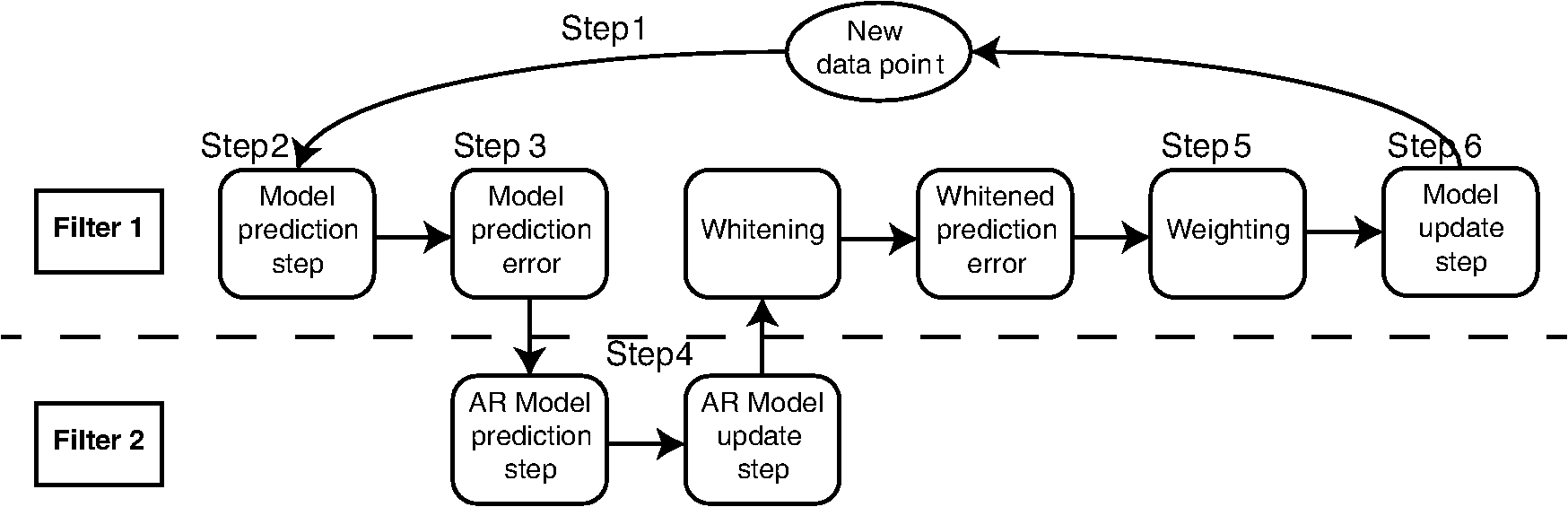

These expressions then yield the update on the estimate of the state ( $β$ ) based on the Kalman implementation of the AR-IRLS model. This estimate is then combined with the next data sample, and steps 1 through 6 are repeated.

2.3.1.

Initializing and tuning the Kalman model

A single Kalman filter contains a total of two tuning parameters ( $R$ and $Q$ ) and two initialization parameters ( $C_{{t = 0}}$ and $β_{{t = 0}}$ ) for the initial values of the state covariance and state estimate, respectively. In our model, the measurement covariance parameter $R$ was replaced by the recursive mean absolute deviation estimator in Eq. (22) and thus is empirically defined by the data. This is the same noise model used in both Kalman filter models. The process noise covariance ( $Q$ ) defines the allowable step-size in the random walk state update model. If $Q$ is large, then $β$ may have large variations from one sample point to the next. In this case, the Kalman gain [ $K_{{t}}$ in Eqs. (11) and (25)] will approach unity, and the estimates of the states will track the innovations term ( $r_{{t}}$ ) and minimize the error to the measurements. In the case that $Q$ is zero, the Kalman estimator will converge onto the static estimate of the state and will asymptotically approach the same solution as the offline analysis model. For a value of $Q$ set between these limits, the Kalman filter will allow some fluctuations in the state. This intermediate tuning is appropriate for real-time tracking of variability of brain activity, for example, in the case of brain–computer interfaces [e.g., Eq. (14)].

In this current work, we have examined only the convergent limit of the Kalman filter where $Q = 0$ for both the GLM and AR Kalman filters (e.g., filters 1 and 2). In particular, in the $Q = 0$ limit, the Kalman filter gain and state update [Eqs. (11)–(13)] reduce to the Bayesian solution of the least-squares regression problem under the assumptions of stationary, white, and independent identically distributed noise and is given by

Eq. (28)

β = C \cdot X^{T} \cdot {(X \cdot C \cdot X^{T} + R)}^{- 1},

where

C

and

R

are the priors on the covariance of

β

and

Y

, respectively, and have the same interpretations as used in the Kalman filter context. Thus, our current implementation performs an online update of the GLM model using the Kalman AR-IRLS model, which approaches the offline (static) solution. In the limit of stationary brain signals, the estimate of the offline and Kalman approaches should be asymptotically comparable. However, if there are nonstationaries in the brain signal, one would expect the Kalman estimator to track these changes and differ from the offline model. This is expected to be true even in the

Q = 0

limit. In the Kalman model, the estimate of the state (e.g., brain activity) at each sample point is thus the maximum likelihood estimate of the state given all the data collected up until that sample. Although a nonzero

Q

implementation, which allows for trial-to-trial variations in the estimate of brain activity, may be more interesting in the context of real-time fNIRS imaging toward feedback or brain–computer interfaces, the

Q = 0

model provides a better means to validate this approach by allowing direct comparison to the offline solution.

The initial values of the states (for both the GLM and AR Kalman filters) were initialized to zero. This means that the initial several time points of the Kalman filter will differ from the static solution until enough data points have been collected to obtain a more precise estimate of the state. In particular, the GLM coefficients will remain zero until after the first instance of the task being performed in the data. In this work, the model is reset to zero after each scan; however, an alternative approach would be to use the last estimates from the previous scan to continue the model. Finally, the initial value of the state covariance ( $C$ ) in our Kalman filter will determine the rate of convergence of the model onto the static solution (since in our model $Q = 0$ ). In this work, we set the initial state covariance to be $100 μ M^{2}$ (e.g., $C_{{t = 0}} = 100 \cdot I$ ).

2.4.

Simulation and Receiver Operating Characteristic Curve Analysis

A resting state fNIRS data set that was acquired as part of a larger study in adults (age 18 to 50, $N = 34$ ) was used for simulation and evaluation of the proposed method’s performance. For each subject, 5 min of resting state data were acquired at 10 Hz sampling frequency. The probe consisted of 35 source–detector pairs with distances between 15 and 31 mm ( $median = 28 mm$ ) and acquired at 690 and 830 nm over the motor and somatosensory cortices.

Simulations were performed by adding a simulated evoked response to real noise from the resting state data (e.g., experimental data recorded during 5 min of rest with no explicit functional task). An evoked response was simulated for a task consisting of a single event every 15 s for 20 trials. A stimulus vector was generated for this task and convolved with a canonical hemodynamic response function and scaled based on contrast-to-noise ratio (CNR). We performed simulations at CNR levels of 0.5, 1.0, and 2.0, in which CNR was defined as the peak magnitude of the response divided by the standard deviation of resting state data after applying a whitening filter. For each set of simulations, data were generated as follows: (1) choose a random channel of resting state data from the pool of all ${HbO}_{2}$ and Hb channels; (2) add a random delay time before the start of the task periods; (3) add a simulated evoked response to the resting state data if desired; and (4) pass the data and design matrix to estimators for assessment of estimated values and statistics. An equal number of simulations were performed on channels with and without adding an evoked response, such that exactly half of all simulations contained a simulated evoked response.

As benchmarks for comparison, the simulated data were also analyzed with two static offline methods: AR-IRLS (Ref. 27) and OLS with AR(1) prewhitening. Comparison with OLS allowed for testing of performance gains over typical OLS-based estimators, and comparison with AR-IRLS allowed for investigation of convergence with the analogous offline method. To evaluate the performance of the estimators, receiver operating characteristic curves (ROCs) were generated using the $t$ -statistic output of the estimators, in which true positive rate is plotted versus the false positive rate (FPR) as a function of the $t$ -statistic threshold for detection of an evoked hemodynamic response. In addition, we compared estimated $p$ values ( $\hat{p}$ ) with actual FPRs. Last, we looked at sensitivity, specificity, and FPR when using $\hat{p} < 0.05$ as the threshold for significance for activation. The simulations were repeated for CNR values of 0.5, 1.0, and 2.0. For estimation with the proposed adaptive method, the process noise covariance $Q$ was set to zero and an $AR (P = 30)$ model was used.

2.5.

Application to Experimental Data

We applied the proposed method to experimental data ( $N = 9$ , age 25 to 47 years) involving a choice reaction time (CRT) task while standing on a fixed force platform or while on a swaying force platform as a final demonstration of the proposed method. The experiment was approved by the institutional review board at the University of Pittsburgh, and all subjects provided written informed consent.

The CRT task has been described in a number of previous publications and is of particular interest as a dual-task model to probe cognitive and balance related interactions. This task has been previously used in a number of behavioral studies.³⁶ Since this task involves standing, balancing, and movement, this task was selected as an example to demonstrate the performance of the proposed motion-correction methods.

In the CRT task, participants were standing and moving on a force platform during the task as shown in Fig. 2. The task involved presentation of an arrow, pointing in the left or right direction, while it was displayed on either the left or right side of the monitor. Subjects were given two response buttons for the left and right hands and were asked to press the button corresponding to the direction of the arrow. Thus, the task consisted of both congruent (left pointing arrow on the left side of the monitor) and incongruent (left pointing arrow on the right side) displays. The paradigm included 10 blocks of 15 s of CRT task followed by 15 s of no task. During the task blocks, new arrows were presented with random direction and location immediately after responding to the previous stimulus until 15 s had elapsed. Each subject performed the task once while standing on a fixed platform and once while the platform was pitching up and down in proportion to the participant’s anterior–posterior body sway. Reaction time and accuracy for each stimulus presented were recorded in addition to NIRS data.

Fig. 2

(a) The probe used for NIRS data acquisition (top and bottom) from two different angles demonstrating typical probe placement. (b) A subject performing a choice reaction time task while balancing on swaying platform. (c) Example of the stimuli, showing incongruent (top) and congruent (bottom) left-pointing arrows. Subjects were asked to respond to the direction of the arrow.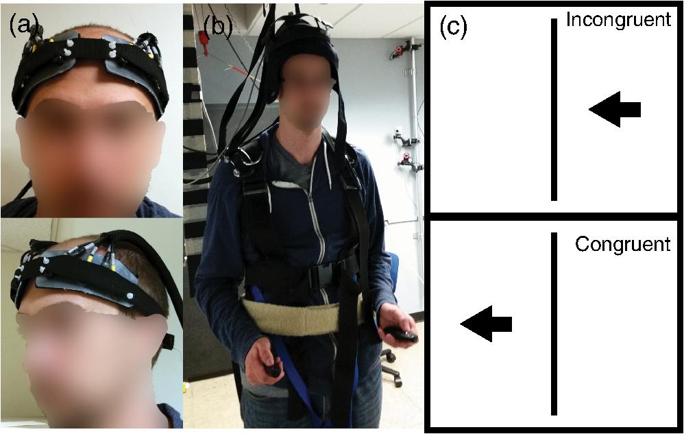

The NIRS data were acquired at 10 Hz on a Techen CW6 system using four source positions ( $690 nm / 830 nm$ ) and six detector positions in a bilateral probe covering the frontal cortex. The source–detector spacing was 3.2 cm, and the probe was centered bilaterally around the 10 to 20 FpZ. The data were then analyzed post hoc using the proposed adaptive method and the offline AR-IRLS method for comparison. The subject level results were used to perform channel-wise group-level analysis via a mixed effects linear model with repeated measures design.

3. Results

3.1.

Simulation Results

An example of the simulated data ( $CNR = 1.0$ ) is shown in Fig. 3. The top panel [Fig. 3(a)] shows a sample time course from the set of experimentally measured resting state data with the simulated evoked stimulus already added to it. Note that the simulated response (which was of magnitude $4 μ M$ in this case) is barely visible on top of the data. Both systemic fluctuations and several motion artifacts are visible in the data trace. Figure 3(b) shows the resulting weight matrix [ $W$ ; Eq. (21)] estimated from this data trace using the adaptive method. The weight function denotes the presence of noise outliers, and thus, when there are sharp changes in the time-series data due to motion, the weight decreases accordingly. This weight matrix is used in the robust regression algorithm to reduce the effects of the heavy-tailed noise in the presence of motion. The states ( $β$ ) of the Kalman filter are shown in Fig. 3(c) along with the true simulated value of the activity. The estimate of $β$ is necessarily zero (the initialized value) until the first stimulus event at around 40 s and then slowly builds up to the level of the true estimate as more data become available in the model. The variations in the state are controlled in the Kalman filter by initial estimate of the state covariance ( $C$ ) and the state process noise ( $Q$ ), which in our model was set to zero ( $Q = 0$ ). Under this limit, the state estimate is expected to approach the value of the static (offline) solution. Note that if $Q$ was set to a higher number, this allows more temporal variability in the state and allows faster convergence of the model. However, a high $Q$ limit, which would then track the measurements more closely by allowing a more volatile state, would not guarantee to converge to the same solution as the offline (static) model and thus prevent direct comparison of the offline and online methods in this work. Figure 3(d) shows the estimate of the $t$ -statistic on the state ( $β$ ), which follows directly from the state and state-covariance terms in the Kalman filter given in Eqs. (26) and (27). At first, the value of the state is close to the initialization value (zero) with high uncertainty, but over time, the $t$ -statistic increases and converges to the offline limit as more data are acquired.

Fig. 3

(a) An example of simulated fNIRS data from resting-state data and synthetic hemodynamic response. (b) Weights calculated by the algorithm. Artifactual time points are down-weighted. (c) The predicted evoked response (solid green) is shown over the simulated evoked response (dashed red). (d) Evolution of the $t$ -statistic over time. Note the difference in scale between (a) and (c). Data are simulated at a contrast-to-noise level of 1:1.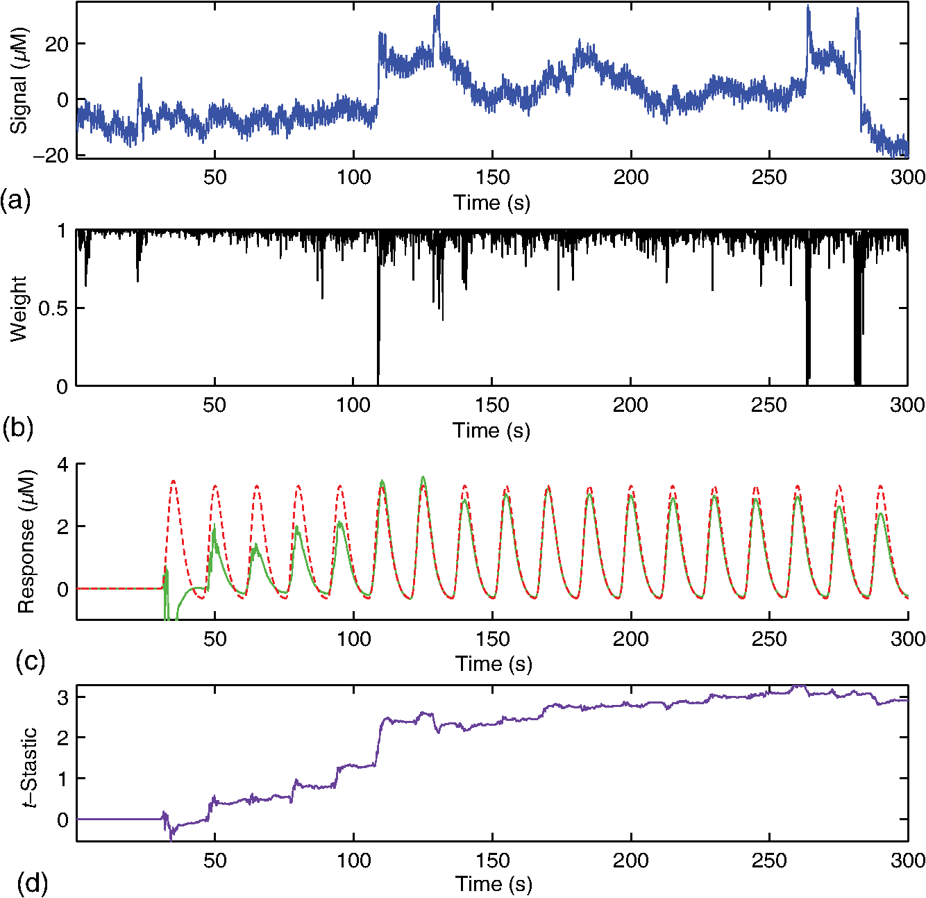

Figure 4 examines the convergent limit of the statistical estimates of $β$ for the Kalman, OLS, and our previous AR-IRLS model. In these simulations, the AR model order ( $P$ ) was varied from 1 to 65 and fit over the same simulated data as previously described using the Kalman, AR(P)-IRLS, and AR(P)-OLS models. This simulation was repeated 1000 times. Figure 4(a) shows the mean statistical effect of the estimate response at the 5 min mark (full data file) for the three models as a function of the AR model order from the 1000 simulations. At low AR order ( $P < 10$ ), the Kalman model had the lowest performance, but above $P > 20$ , the model had similar performances (within 10% variations). For the Kalman model, only model orders below $P < 20$ were statistically different ( $p < 0.05$ ) from the value obtained at order $P = 65$ . Thus, our selection of $P = 30$ seemed justified. In Figs. 4(b) and 4(c), the correlation of the $t$ -statistics for these three models is compared at $P = 1,30$ , and 50. The best-fit lines of the comparison of the AR-OLS and AR-IRLS models were $R = 0.68, 0.77$ , and 0.72 for $P = 1,30$ , and 50, respectively. The slope less than unity indicates that the effect size of the OLS model tended to be higher than the IRLS model. However, this comparison only looks at the magnitude of the effect size, and our previous work has also shown that the OLS model has a higher FDR. This is examined in Sec. 3.2 and Fig. 5. The comparison of the AR-IRLS and Kalman model had best-fit slopes of $R = 1.24$ , 1.07, and 1.06. Here, a value greater than unity indicates the AR-IRLS model had higher effect sizes on average than the Kalman model. However, this was only significantly different for the $P = 1$ model ( $p < 1 e - 7$ ).

Fig. 4

The performance of the AR-IRLS, AR-OLS, and Kalman models was examined as a function of the AR model order ( $P$ ). 1000 simulations were generated at a CNR of 1.0 and estimated using the three approaches at model orders from 1 to 65. (a) The average (and standard errors) of the 1000 simulations at each AR model order. (b) and (c) Scatter plots of the individual results from the $P = 1, 30$ , and 50 models for the comparison of the AR-IRLS/AR-OLS and AR-IRLS/Kalman models, respectively. The best-fit lines are also presented.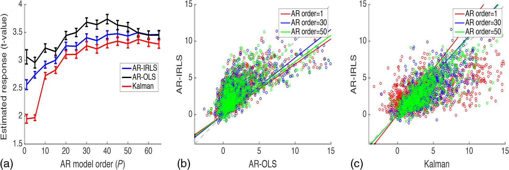

Fig. 5

ROC curves are shown for 1, 2, 3, 4, and 5 min of data. The statistical performance proposed adaptive method converted rapidly to the analogous offline AR-IRLS method. The top row shows the true positive rate (TPR) plotted against FPR. The bottom row shows the FPR plotted versus the uncontrolled estimate of the probability value ( $\hat{p}$ ). Data are simulated at a contrast-to-noise level of 1:1 as exemplified in Fig. 3.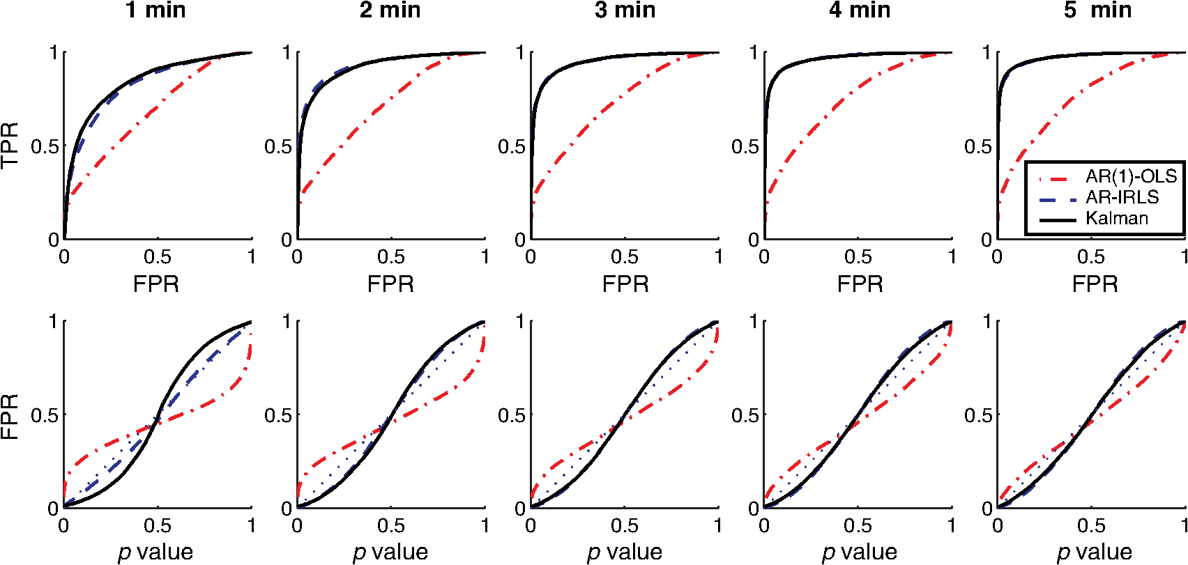

Simulations similar to the one shown in Fig. 3 were repeated from the sample of 34 subjects’ resting state data to generate ROCs to quantify the performance of the model. In Fig. 5, we show the ROCs generated using the first 1 through 5 min of data. Both the Kalman filter (solid black) and offline (dotted black) models are shown. The two lines are virtually identical and indistinguishable except for the 1-min window. The offline analysis used the same 1 to 5 min block of data. Also shown is the AR(1)-OLS regression model, which does not use robust regression for comparison. In our previous work, we had already shown that this OLS model was inferior to the robust regression version of the model.²⁷ In the top row, we show the sensitivity–specificity curves for the models based on 1 to 5 min of data. Not surprisingly, as the amount of data is increased, the area under the curve (AUC) of the ROC plots increases and asymptotes around 3 to 4 min. Figure 6 presents the comparison of these AUC values in terms of the sensitivity and specificity of these plots at $\hat{p} < 0.05$ . The proposed adaptive method shows a performance similar to the analogous offline AR-IRLS method. Both of the methods showed increased performance with increasing data length. These two methods show slight divergence early on (using only 1 min of data) due to the lead-in period of the Kalman estimator. Beyond 2 min, however, the offline and online methods show nearly identical performance. Both of these methods showed better performance than the OLS method. In the lower row of Fig. 5, we show the estimate of the FPR based on the $t$ -statistic reported from the models compared to the actual FPR from the ROC analysis. In particular, in our previous work in Ref. 27, we had shown that presence of serial correlations in the noise led to large differences between the reported ( $\hat{p}$ ) and actual FDRs. An ideal model would have the reported and actual rates equal as indicated by a line at slope of one. In agreement with our previous work, we found that prewhitening with the $AR (p)$ model produced the least biased estimates of the FDRs. The adaptive (Kalman) and offline produced similar results with a slight deviation using only the first minute of data. This is presumably due to the lead in time of the AR Kalman filter model (filter #2 in Fig. 1). These values are also presented in Fig. 6(c) at the expected $\hat{p} < 0.05$ threshhold. By definition, at a threshold of $\hat{p} < 0.05$ , the FDR ( $FDR = 1$ -specificity) is expected to be 5%. Deviations from this expected rate indicate uncontrolled or overcontrolled type I errors in the model as detailed in Ref. 33. In these results, at this threshold, the actual FDR of the OLS model is under-reported with a value between $FDR = [0.1, 0.2]$ . This means that data reported using this offline OLS model have about two to four times more false positives than expected. The offline and Kalman $AR (p)$ -IRLS models both slightly over-reported FDRs, meaning that the results were actually more significant than expected (e.g., the model slightly overcorrects). This finding had also been reported in the original paper by Barker et al.²⁷

Fig. 6

(a) Sensitivity, (b) specificity, and (c) FPR are shown for simulated data using $\hat{p} < 0.05$ as the threshold for activation. These data are also presented as an ROC curve in Fig. 5 and were simulated at a contrast-to-noise level of 1:1.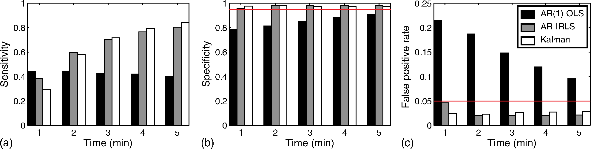

The results for the $CNR = 0.5$ , 1.0, and 2.0 simulations for the Kalman $AR (p)$ -IRLS model are additionally provided in Table 1. The lower $CNR (= 0.5)$ results had roughly half the sensitivity at all five time windows compared to the $CNR = 1.0$ data presented in Figs. 5 and 6. Likewise, the $CNR = 2.0$ data had about twice the sensitivity of the data. This was expected based on the definition of the CNR. Note these three CNR levels correspond to Cohen’s $d$ values around 0.3, 0.7, and 1.4 per trial, which are small, medium, and moderate effect sizes. In comparison, the experimental CRT data had a Cohen’s $d$ of around $d = 0.5$ per trial for the most activated channels, which was slightly lower than the $CNR = 1$ simulations shown in Figs. 3–6.

Table 1

Sensitivity, specificity, and FPR are shown for varying CNRs for the proposed algorithm using p^<0.05 as the threshold for activation. Specificity is equal to 1 — FPR. Sensitivity is equal to the true positive rate. The offline results for the full 5 min of simulation from the OLS and AR-IRLS models are also presented.

	Kalman model					AR-OLS	AR-IRLS
	1 min	2 min	3 min	4 min	5 min	5 min	5 min
Sensitivity \| True positive rate
$SNR = 0.5$	10.8%	28.4%	40.1%	49.3%	56.0%	21.2%	43.5%
$SNR = 1.0$	29.5%	57.7%	71.6%	79.4%	84.0%	40.4%	80.2%
$SNR = 2.0$	57.9%	82.6%	91.7%	95.1%	96.5%	65.5%	94.5%
Specificity
$SNR = 0.5$	97.6%	97.9%	97.4%	97.3%	97.2%	91.3%	98.3%
$SNR = 1.0$	97.6%	97.7%	97.3%	97.3%	97.1%	88.2%	98.3%
$SNR = 2.0$	97.5%	97.7%	97.3%	97.3%	97.2%	88.4%	98.5%
False positive rate
$SNR = 0.5$	2.4%	2.1%	2.6%	2.7%	2.8%	8.7%	1.7%
$SNR = 1.0$	2.5%	2.3%	2.7%	2.7%	2.9%	11.8%	1.7%
$SNR = 2.0$	2.5%	2.3%	2.7%	2.7%	2.8%	11.6%	1.5%

3.2.

Estimation of Dynamic States

In the simulations shown for Figs. 3–6, we examined the performance of the Kalman estimate in the low- $Q$ limit for estimating a static brain signal. We showed that this produced a convergent solution to the offline analysis model but allowed the additional benefit of an online cumulative estimate of the brain activity that could be shown during actual data collection. The alternative high- $Q$ limit of a Kalman filter, in principle, allows estimation of time-varying and dynamic states (brain activity) and could be used in brain–computer interfaces based on Kalman estimators (e.g., Ref. 14). To examine the performance of our model under these limits, we performed an additional set of simulations where trial-by-trial variability in the hemodynamic response was introduced. Figure 7(a) shows an example of such simulations. For each simulation, the magnitude of the evoked response for each trial was given as $β_{0} \pm Δ β$ , where $Δ β \in N (0, Q_{B})$ and $β_{0}$ is defined to give a specific average contrast-to-noise value of 1.0 for each data file. Figure 7(b) shows the simulated response at $Q_{B} = 10 μ M^{2}$ , which is a large inter-trial variability and displays both changes in amplitude and sign reversals of the response (red line). The recovered estimates from the Kalman filter model for this particular simulation is shown at $Q = 0 μ M^{2}$ (black dotted line) and $Q = 50 μ M^{2}$ (black solid line) in Fig. 7(b). As can be seen, the $Q = 0$ model tracks some of the variability in the response but has overall poor performance, and the estimate remains close to the mean of the average trial response (which is close to zero since about half the responses have negative amplitude). In the high- $Q$ limit, the Kalman model does a better job of tracking the simulated inter-trial variability. The estimated responses for multiple $Q$ values within the range of $Q = 0$ to $50 μ M$ is additionally shown in Fig. 7(c), which demonstrates the progression from a fairly static estimate to a fully dynamic state estimate as a function of the increasing Kalman state process noise ( $Q$ ).

Fig. 7

The performance of the Kalman model was examined for increasing levels of inter-trial variability in the simulated brain activity to investigate the use of the model for estimating nonstationary brain signals. (a) An example of a simulated data trace is shown for an inter-trial variance of $Q_{B} = 10 μ M^{2}$ [also indicated by the vertical white dotted line in (d) and (e)]. (b) The simulated response (Truth) is shown and also the estimates of this response using a Kalman model with low $Q$ ( $Q = 0 μ M^{2}$ ) and high $Q$ ( $Q = 50 μ M^{2}$ ). (c) Additional levels of $Q$ from 0 to $50 μ M^{2}$ are provided, demonstrating the transition from nearly static to dynamic state estimate. The $y$ -axis indicates the state noise ( $Q$ ) used in each recovery, and each signal is shown with a dc-shift to indicate the noise prior and plotted with the same linear vertical scale for each line to allow comparison. These simulations were repeated 500 times at each of the 11 levels of inter-trial variance ( $Q_{B}$ from 0 to $50 μ M^{2}$ ), and the average is presented in (d). (d) The contour map of the $R^{2}$ comparison of the recovered estimate of trial-by-trial variations in the brain signal and the simulated response as a function of the Kalman process noise ( $Q$ ; $y$ -axis) and the simulated variability ( $Q_{B}$ ; $x$ -axis). The static AR-IRLS estimate as a function of the simulated variability is shown in (e). Data are simulated at a (mean contrast)-to-noise ratio of 1:1.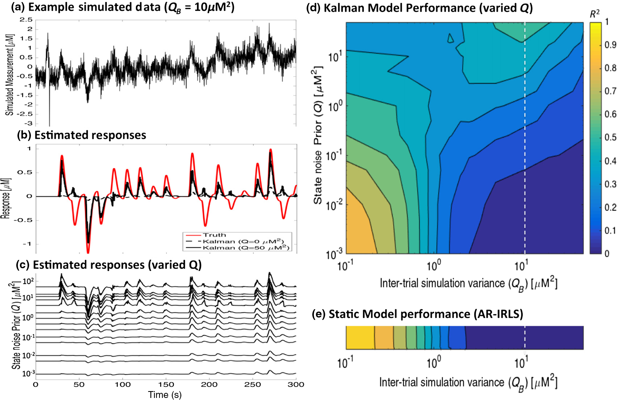

Figures 7(a)–7(c) demonstrate one such example simulation, but to investigate this in more detail, the variance of the trials ( $Q_{B}$ ) was simulated at 15 increasing levels from stationary ( $Q_{B} = 0 μ M^{2}$ ) to highly dynamic ( $Q_{B} = 50 μ M^{2}$ ). The Kalman model was then run at 11 differing levels of state process noise ( $Q$ ) from the low- $Q$ ( $Q = 0 μ M^{2}$ ) to high- $Q$ ( $Q = 50 μ M^{2}$ ) limit. This simulation was repeated 500 times for each combination. In Fig. 7(d), we show the $R^{2}$ model comparison between the simulated inter-trial variability and the recovered estimate from the ( $Z$ -transformed) average of the 500 simulations at each of the 165 combinations of $Q$ and $Q_{B}$ . For comparison, the results of the static model at each of these $Q_{B}$ values are shown in Fig. 7(e). As can be seen for both the static and low- $Q$ Kalman filter cases, the model performance falls off as inter-trial variance increases. At $Q_{B} = 10 μ M$ (indicated in the dotted white vertical line), which matches the simulations shown in Figs. 7(a)–7(c), the static and low- $Q$ Kalman models have nearly zero performance ( $R^{2} < 0.1$ ). In the Kalman filter, however, this performance can be slightly recovered by increasing the process noise ( $Q$ ) of the model and can partly model even large inter-trial variability, which agrees with the single demonstration shown in Fig. 7(b). However, in this range, the Kalman model has lower overall performance ( $R^{2} \sim 0.4$ to 0.5). Furthermore, at higher $Q$ , the Kalman model loses sensitivity to static responses (e.g., $Q_{B} = 0$ ), so selecting a high $Q$ in the absence of inter-trial variability in the brain response is quite detrimental.

4. Experimental Results

Experimental fNIRS data were collected on nine volunteers during the CRT-balance task and analyzed post hoc using both the proposed Kalman filter and off-line (static) $AR (p)$ -IRLS models. Figure 8 shows the comparison of the estimated coefficients ( $β$ ; top row) and the $t$ -statistics (bottom row) for the adaptive and static models. The comparisons are shown using the first 1 through 5 min (entire data). These scatter plots show the correlation between the offline and Kalman models. Each point represents the estimate for one of the fNIRS source–detector pairs for one of the subjects. As expected from the simulations, initially, there is some mismatch between the two methods as suggested by the slope of the regression lines at the 1 min mark due to the time needed for the adaptive algorithm to converge. Because the covariance matrix is typically initialized with a large covariance ( $C_{{t = 0}} = 100 \cdot I$ ), the $t$ -statistics were initially underestimated as demonstrated by a slope value smaller than 1 until the adaptive algorithm converged. By the end of the scan (5 min), the slopes of the regression lines for the coefficients and $t$ -statistics converged to values close to one, suggesting that there are no systematically different biases between the estimators. Both Pearson’s correlation ( $R$ ) and Spearman’s correlation ( $ρ$ ) between the results of the two estimators increased over time with more data. Above 3 min of data, the slope of the line comparing the two models for both the $t$ -statistic and coefficients is close to unity, indicating that the two models agreed with each other on average. However, there was quite a bit of variation around this slope, indicating that the data probably did have some nonstationaries in the brain response, which were being modeled by the adaptive Kalman filter but not the static model.

Fig. 8

Comparison of (a) coefficient (beta) and (b) $t$ -statistics for the offline (AR-IRLS) and online (Kalman) analysis methods across all channels of ${HbO}_{2}$ for all subjects using varying lengths of the time-series data from 1 to 5 min. Each point indicated by a “ $+$ ” symbol represents a source–detector pair for one of the subjects and for one of the conditions (sway or fixed platform). The solid black line indicates regression line indicating the relationship between the online Kalman estimates and the offline AR-IRLS estimates. The dashed red line indicates the ideal regression line with a slope of one. A difference in slopes between the red and black lines indicates systematic difference between the two estimators.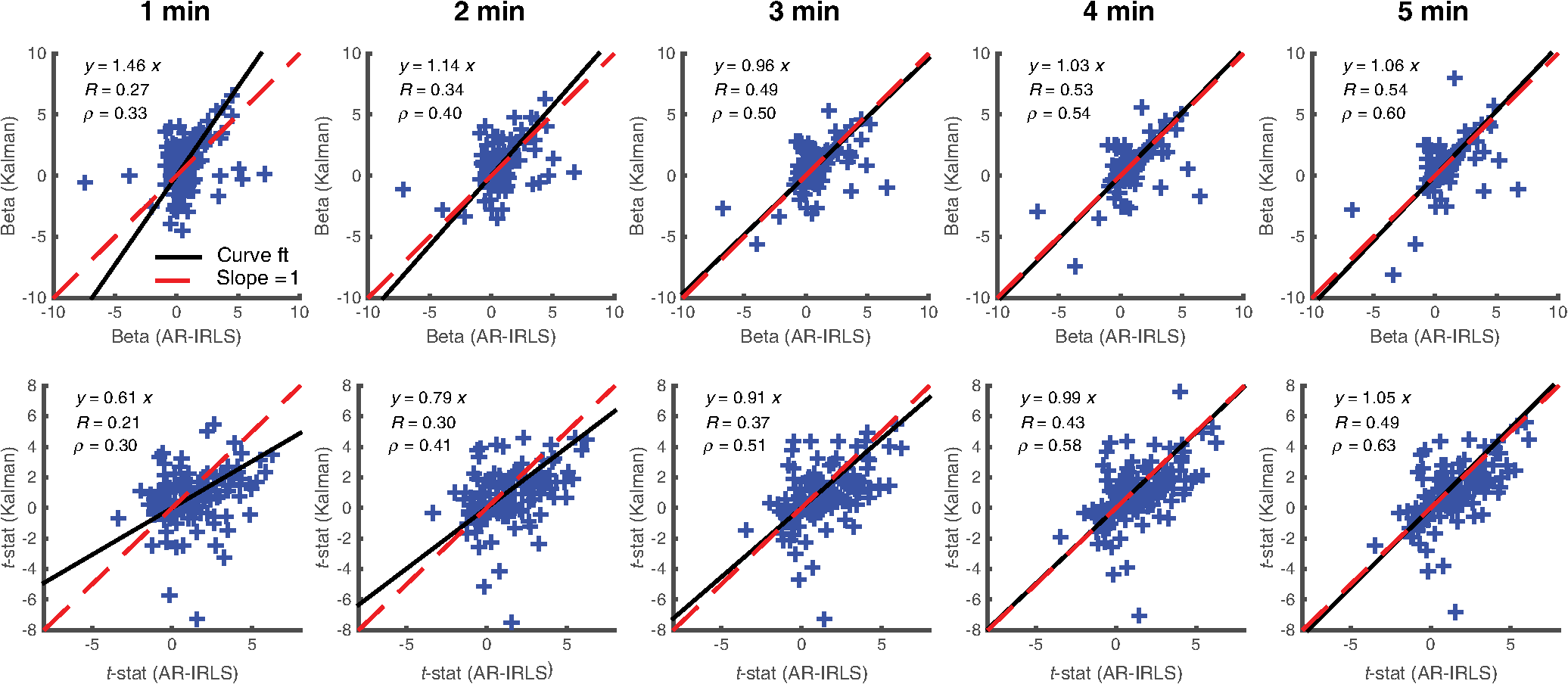

Finally, Fig. 9 shows the results for group-level analysis using the subject-level results from the proposed online Kalman filtering method as well as the offline AR-IRLS method. Both methods show activation in the right frontal cortex for the CRT task under both the fixed platform and swaying platform conditions.

Fig. 9

Group-level statistics for ${HbO}_{2}$ using subject-level statistics from the (a) offline (AR-IRLS) and (b) online (Kalman) analysis methods. Thick lines indicate activation at a significance level of $\hat{p} < 0.05$ (uncorrected) and are shown overlain on an atlas structural image based on the registration of the fNIRS probe to the FpZ 10-20 coordinate.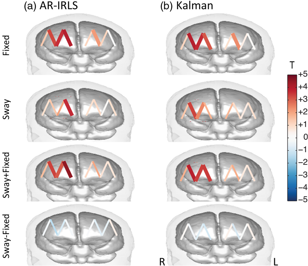

For the CRT response on fixed platform, the static and Kalman filtering models produced similar results and activation patterns as shown in Fig. 9. In the sway condition (where the floor platform moves during the CRT task), the Kalman filter model showed more significant activation on the right hemisphere compared to the static model. Although this difference was not statistically different between the two models, it could indicate that the CRT response during sway had higher single-trial variability (e.g., nonstationarity), which was better modeled by the adaptive Kalman method.

No significant differences were detected in the hemodynamic response to the task between standing on a fixed versus a swaying platform for either the static or Kalman filtering model. In both models, the CRT response while on the fixed surface was larger than the swaying platform, which is consistent with a dual-task interference effect, although this difference was not statistically significant for any channels.

5. Discussion

In this study, we have developed methods for adaptive estimation of the GLM based on using two Kalman filters: one to estimate the model and one to estimate an AR model of the residual error. Before the update step of the first Kalman filter, the model is whitened based on the AR coefficients of the second Kalman filter and weighted by a weighting function. This mitigates the effects of serial correlations and outliers on the estimator. The proposed method was compared to an analogous offline algorithm (AR-IRLS) that implements the same concepts. The proposed online method showed very similar performance to the AR-IRLS method for offline processing. Last, we demonstrated the method on an experimental data set, in which the online and offline methods showed good agreement.

5.1.

Simulation Results

In the first half of this work, we provided simulation results that showed similar performance of the static and Kalman filtering models in terms of sensitivity, specificity, and control for type I errors. In the implementation used in this work, we set the state process noise ( $Q$ ) to zero in the model. Under this limit, the Kalman filter performs an optimal data integrator and converges to the static solution for the estimate of the states. The $Q = 0$ model thus produces a running estimate of the GLM model coefficients based on the data collected up until the current sample point. In this mode, the low- $Q$ Kalman filter can be thought of as an optimal cumulative integrator and estimates the weighted-average response of all trials up to the current time point. This model assumes a static probability distribution function on the state estimate. This still allows some inter-trial variations in the response estimate when the underlying brain signal is nonstationary but converges to the static offline solution in the case of time-invariant signals. Using this model, one is able to estimate the brain activity during data collection and obtain a solution similar to that obtained in offline analysis. In particular, the current Kalman filter implementation reports statistical values and control for type I error, which is similar to our previous AR-IRLS model.²⁷ First, this current model provides better control for the type I errors compared to the OLS version of the GLM model used in the Kalman filter developed by Abdelnour and Huppert.¹⁴ Similar to the performance of this model in the static (offline) implementation described in Ref. 27, the AR prewhitening filter allows correction of the serially correlated errors due to systemic physiology. Without correction, these correlations lead to overestimation of the effective degrees of freedom within the data and can result in high FDRs. Second, the implementation of robust regression methods within the model allows better rejection of motion artifacts as heavy-tailed outliers in the noise distribution.

The Kalman filter framework also allows for time-varying states when $Q$ is nonzero. This may be useful for investigating inter-trial variance or for applications where the evoked response is expected to be modulated, such as by learning or habituation. In previous work by Abdelnour and Huppert,¹⁴ a similar Kalman filtering implementation of the OLS regression model was developed and applied to real-time estimation of brain activity in the motor cortex. In that work, the nonzero $Q$ implementation of the Kalman filter was used to track changes in brain activity. This model used the timing of task events to define the GLM but allowed the state to dynamically vary over time. In particular, subjects directed a brain–computer interface by moving their left or right hand, allowing the Kalman filter to track these changes in the level of brain activity in the left and right motor areas of the brain. In Fig. 7, we investigated the performance of our proposed model in the presence of trial-to-trial variability in the brain response. We found that the low- $Q$ Kalman and static offline solutions provided similar model fits. When the underlying brain signals were static (no inter-trial variability), both models had good performance ( $R^{2} > 0.9$ for the $CNR = 1$ case), but the performance of both models decreases with added inter-trial variability. Increasing the process noise ( $Q$ ) in the Kalman filter was able to partially recover the performance at high inter-trial variability, although the overall performance ( $R^{2} \sim 0.3$ to 0.5) was diminished from the case of no simulated inter-trial variability. This is not surprising since when process noise is too large, the Kalman filter will overfit noise in the time series by allowing large dynamic changes in the states. This suggests that a low $Q$ value for the Kalman filter is preferable unless there is strong evidence of brain activity nonstationarity or if inter-trial variability is of specific interest in the study (e.g., brain–computer interfaces or modeling neural habitation). We also note that in this paper, we the state process noise tuning with constant AR model order ( $P = 30$ ). Although we showed that the model order had little effect above critical order, we did not look at the interactions between model order and state process noise in the context of capturing inter-trial variability and should be examined in future studies.

5.2.

Experimental Results

In the experimental example, we applied this model to a brain imaging task involving measurements of postural sway during a dual-task choice reaction time (CRT) task. For a review on the role of the CRT task in aging research, see Ref. 37. This task was chosen as a demonstration because it highlights the ability to image the brain during movement studies, which is one of the advantages of fNIRS over other methods like fMRI. This is also one of the more challenging experimental scenarios for fNIRS because of the presence of motion artifacts associated with postural changes and physical movement. In this data, we looked at evoked brain activity to the CRT task while standing on a fixed and a swaying platform. In both conditions, we found activation on the right frontal cortex.

Similar to the simulation results, the Kalman filter model produced results similar to the offline analysis using the AR-IRLS model. As demonstrated by the scatter plots in Fig. 8, there were no significant biases between these two models in terms of either the estimate of the state ( $β$ ) or the statistical $t$ -test. However, as noted in Figs. 8 and 9, there were per-channel and subject variations between these two models. In particular, the Kalman filter provides an adaptive estimate of the brain activity. In the limit that the underlying state is stationary (as in the case of our simulated data), the offline (static) model and Kalman estimator with $Q = 0$ will converge to the same solution. This statement, however, is only true when the underlying brain activity is static (e.g., there is no trial-by-trial variability in the brain response). In the case of physiological variability in the brain response, the Kalman filter will allow better tracking of these changes compared to the static linear model even under the limit of $Q = 0$ .

In the experimental data, we found similar estimates of brain activity during the CRT task on the fixed platform for the Kalman and static AR-IRLS model. However, in the sway condition, we found greater effect sizes in the Kalman filtering model. This could indicate greater trial-by-trial variability in the brain activity under this condition, which could explain the increased performance of the Kalman model compared to the static solution.

Both the static and Kalman models showed increased brain activity in the right frontal region during the CRT task. This result is consistent with previous studies using similar choice reaction tasks showing involvement in the right dorsal lateral prefrontal cortex.³⁸ During the sway condition, there was a decrease (albeit not statistical) in the CRT response compared to the fixed platform condition. Previous dual-task studies using a similar CRT have demonstrated decreased task performance during the balance task, particularly in older populations.³⁷^,³⁹ In particular, it is believed that choice reaction time slows with aging and with increased task difficulty, which allegedly reflects competition for attentional resources (reviewed in Ref. 37). In this study, which used only younger participants, we did not find any statistical changes in the reaction time for subjects on the fixed versus swaying platform. This could explain why we also failed to observe significant differences in the brain responses under these two conditions.

5.3.

Extensions of Model

One significant difference between the online and offline algorithms is that the AR-IRLS method employs a model selection step using BIC (Ref. 40) to choose an optimal AR model order. However, this step is not possible in the current real-time implementation, which instead used fixed AR model order (in this case, $P = 30$ ). Our simulation results show that choosing an appropriate model order beforehand did not significantly degrade the performance and that the model was stable for a range of order selections above some critical order (see Fig. 4). In future work, it may be possible to implement a model selection variation of the second (AR model) Kalman estimator by running in parallel several of these filters differing in the AR model order and using the same criterion, such as BIC, to select the best model. Additional testing is needed to validate such an approach.

6. Conclusions

Potential applications of real-time imaging include the development of brain–machine interfaces,²²^,²³ monitoring attentional states,⁴¹ providing bedside feedback in clinic,⁴² and the investigation of neurofeedback.⁴³ We validated this method by performing ROC analysis on simulations using simulated evoked hemodynamics added to experimental resting-state NIRS data. The resting-state NIRS data acted as real noise with contributions from physiology, motion, and instrument noise. Last, we applied the proposed method post hoc to an fNIRS study of a cognitive reaction time task during a standing balance task and compared the adaptive estimation with the conventional static linear estimation model. We found that the algorithm offers adaptive estimation of fNIRS data that is suitable for real-time application and is robust to serial correlations from physiology and outliers from motion.

In conclusion, we developed a new method for adaptive estimation of the GLM that is robust to motion artifacts and systemic physiology. The new method showed performance similar to the offline AR-IRLS algorithm. The method shows better performance than OLS type methods in both sensitivity and type I error control. Finally, since the method is adaptive, it is suitable for real-time analysis of fNIRS data.

Acknowledgments

This study was supported by the National Institutes of Health (Grants R01EB013210 and P30AG024827).

References

1.

F. F. Jobsis, “Noninvasive, infrared monitoring of cerebral and myocardial oxygen sufficiency and circulatory parameters,” Science, 198 (4323), 1264 –1267 (1977). http://dx.doi.org/10.1126/science.929199 SCIEAS 0036-8075 Google Scholar

2.

M. Cope et al., “Methods of quantitating cerebral near infrared spectroscopy data,” Adv. Exp. Med. Biol., 222 183 –189 (1988). http://dx.doi.org/10.1007/978-1-4615-9510-6 AEMBAP 0065-2598 Google Scholar

3.

J. Steinbrink et al., “Illuminating the BOLD signal: combined fMRI-fNIRS studies,” Magn. Reson. Imaging, 24 (4), 495 –505 (2006). http://dx.doi.org/10.1016/j.mri.2005.12.034 Google Scholar

4.

I. Miyai et al., “Cortical mapping of gait in humans: a near-infrared spectroscopic topography study,” NeuroImage, 14 (5), 1186 –1192 (2001). http://dx.doi.org/10.1006/nimg.2001.0905 NEIMEF 1053-8119 Google Scholar

5.

M. Suzuki et al., “Activities in the frontal cortex and gait performance are modulated by preparation. An fNIRS study,” NeuroImage, 39 (2), 600 –607 (2008). http://dx.doi.org/10.1016/j.neuroimage.2007.08.044 NEIMEF 1053-8119 Google Scholar

6.

H. Karim et al., “Functional brain imaging of multi-sensory vestibular processing during computerized dynamic posturography using near-infrared spectroscopy,” NeuroImage, 74 318 –325 (2013). http://dx.doi.org/10.1016/j.neuroimage.2013.02.010 NEIMEF 1053-8119 Google Scholar

7.

H. Karim et al., “Functional near-infrared spectroscopy (fNIRS) of brain function during active balancing using a video game system,” Gait Posture, 35 (3), 367 –372 (2012). http://dx.doi.org/10.1016/j.gaitpost.2011.10.007 Google Scholar

8.

H. T. Karim et al., “Neuroimaging to detect cortical projection of vestibular response to caloric stimulation in young and older adults using functional near-infrared spectroscopy (fNIRS),” NeuroImage, 76 1 –10 (2013). http://dx.doi.org/10.1016/j.neuroimage.2013.02.061 NEIMEF 1053-8119 Google Scholar

9.

X. Cui, D. M. Bryant and A. L. Reiss, “NIRS-based hyperscanning reveals increased interpersonal coherence in superior frontal cortex during cooperation,” NeuroImage, 59 (3), 2430 –2437 (2012). http://dx.doi.org/10.1016/j.neuroimage.2011.09.003 NEIMEF 1053-8119 Google Scholar

10.

C. Bogler et al., “Decoding vigilance with NIRS,” PLoS One, 9 (7), e101729 (2014). http://dx.doi.org/10.1371/journal.pone.0101729 Google Scholar

11.

M. Aqil et al., “Cortical brain imaging by adaptive filtering of NIRS signals,” Neurosci. Lett., 514 (1), 35 –41 (2012). http://dx.doi.org/10.1016/j.neulet.2012.02.048 NELED5 0304-3940 Google Scholar

12.

X. Wang et al., “Real-time continuous neuromonitoring combines transcranial cerebral Doppler with near-infrared spectroscopy cerebral oxygen saturation during total aortic arch replacement procedure: a pilot study,” ASAIO J., 58 (2), 122 –126 (2012). http://dx.doi.org/10.1097/MAT.0b013e318241abd3 Google Scholar

13.

X. S. Hu et al., “Kalman estimator- and general linear model-based on-line brain activation mapping by near-infrared spectroscopy,” Biomed. Eng. Online, 9 82 (2010). http://dx.doi.org/10.1186/1475-925X-9-82 Google Scholar

14.

A. F. Abdelnour and T. Huppert, “Real-time imaging of human brain function by near-infrared spectroscopy using an adaptive general linear model,” Neuroimage, 46 (1), 133 –143 (2009). http://dx.doi.org/10.1016/j.neuroimage.2009.01.033 NEIMEF 1053-8119 Google Scholar

15.

C. Soraghan et al., “A 12-channel, real-time near-infrared spectroscopy instrument for brain-computer interface applications,” in Annual Int. Conf. of the IEEE Engineering in Medicine and Biology Society, 5648 –5651 (2008). http://dx.doi.org/10.1109/IEMBS.2008.4650495 Google Scholar

16.

F. Matthews et al., “Software platform for rapid prototyping of NIRS brain computer interfacing techniques,” in Annual Int. Conf. of the IEEE Engineering in Medicine and Biology Society, 4840 –4843 (2008). http://dx.doi.org/10.1109/IEMBS.2008.4650297 Google Scholar

17.

Y. Shingu et al., “Real-time cerebral monitoring using multichannel near-infrared spectroscopy in total arch replacement,” Jpn. J. Thorac. Cardiovasc. Surg., 51 (4), 154 –157 (2003). http://dx.doi.org/10.1007/s11748-003-0052-1 Google Scholar

18.

N. Birbaumer et al., “Neurofeedback and brain-computer interface clinical applications,” Int. Rev. Neurobiol., 86 107 –117 (2009). http://dx.doi.org/10.1016/S0074-7742(09)86008-X Google Scholar

19.

U. Chaudhary, N. Birbaumer and M. R. Curado, “Brain-machine interface (BMI) in paralysis,” Ann. Phys. Rehabil. Med., 58 (1), 9 –13 (2015). http://dx.doi.org/10.1016/j.rehab.2014.11.002 Google Scholar

20.

S. Fazli et al., “Using NIRS as a predictor for EEG-based BCI performance,” in Annual Int. Conf. of the IEEE Engineering in Medicine and Biology Society, 4911 –4914 (2012). http://dx.doi.org/10.1109/EMBC.2012.6347095 Google Scholar

21.

S. Fazli et al., “Enhanced performance by a hybrid NIRS-EEG brain computer interface,” NeuroImage, 59 (1), 519 –529 (2012). http://dx.doi.org/10.1016/j.neuroimage.2011.07.084 Google Scholar

22.

R. Sitaram et al., “Temporal classification of multichannel near-infrared spectroscopy signals of motor imagery for developing a brain-computer interface,” NeuroImage, 34 (4), 1416 –1427 (2007). http://dx.doi.org/10.1016/j.neuroimage.2006.11.005 NEIMEF 1053-8119 Google Scholar

23.

S. M. Coyle, T. E. Ward and C. M. Markham, “Brain–computer interface using a simplified functional near-infrared spectroscopy system,” J. Neural Eng., 4 (3), 219 –226 (2007). http://dx.doi.org/10.1088/1741-2560/4/3/007 Google Scholar

24.

N. Birbaumer et al., “Physiological regulation of thinking: brain–computer interface (BCI) research,” Prog. Brain Res., 159 369 –391 (2006). http://dx.doi.org/10.1016/S0079-6123(06)59024-7 Google Scholar

25.

M. A. Yucel et al., “Reducing motion artifacts for long-term clinical NIRS monitoring using collodion-fixed prism-based optical fibers,” NeuroImage., 85 (Pt 1), 192 –201 (2014). http://dx.doi.org/10.1016/j.neuroimage.2013.06.054 Google Scholar

26.

S. Brigadoi et al., “Motion artifacts in functional near-infrared spectroscopy: a comparison of motion correction techniques applied to real cognitive data,” NeuroImage, 85 (Pt 1), 181 –191 (2014). http://dx.doi.org/10.1016/j.neuroimage.2013.04.082 Google Scholar

27.

J. W. Barker, A. Aarabi and T. J. Huppert, “Autoregressive model based algorithm for correcting motion and serially correlated errors in fNIRS,” Biomed. Opt. Express, 4 (8), 1366 –1379 (2013). http://dx.doi.org/10.1364/BOE.4.001366 Google Scholar

28.

R. J. Cooper et al., “A systematic comparison of motion artifact correction techniques for functional near-infrared spectroscopy,” Front. Neurosci., 6 147 (2012). http://dx.doi.org/10.3389/fnins.2012.00147 Google Scholar

29.

L. Gagnon et al., “Further improvement in reducing superficial contamination in NIRS using double short separation measurements,” NeuroImage, 85 (Pt 1), 127 –135 (2014). http://dx.doi.org/10.1016/j.neuroimage.2013.01.073 Google Scholar

30.

T. J. Huppert et al., “HomER: a review of time-series analysis methods for near-infrared spectroscopy of the brain,” Appl. Opt., 48 (10), D280 –D298 (2009). Google Scholar

31.

C. Matteau-Pelletier et al., “1/f noise in diffuse optical imaging and wavelet-based response estimation,” IEEE Trans. Med. Imaging, 28 (3), 415 –422 (2009). http://dx.doi.org/10.1109/TMI.2008.2006524 ITMID4 0278-0062 Google Scholar

32.

R. E. Kalman, “A new approach to linear filtering and prediction problems,” J. Fluids Eng., 82 (1), 35 –45 (1960). http://dx.doi.org/10.1115/1.3662552 JFEGA4 0098-2202 Google Scholar

33.

T. J. Huppert, “Commentary on the statistical properties of noise and its implication on general linear models in functional near-infrared spectroscopy,” Neurophotonics, 3 (1), 010401 (2016). http://dx.doi.org/10.1117/1.NPh.3.1.010401 Google Scholar

34.

P. W. Holland and R. E. Welsch, “Robust regression using iteratively reweighted least-squares,” Commun. Stat. Theory Methods, 6 (9), 813 –827 (1977). http://dx.doi.org/10.1080/03610927708827533 Google Scholar

35.

A. E. Beaton and J. W. Tukey, “The fitting of power series, meaning polynomials, illustrated on band-spectroscopic data,” Technometrics, 16 (2), 147 –185 (1974). http://dx.doi.org/10.1080/00401706.1974.10489171 TCMTA2 0040-1706 Google Scholar

36.

A. Rodriguez et al., “Regional oxygen saturation index (

{rSO}_{2}

) in brachioradialis and deltoid muscle. Correlation and prognosis in patients with respiratory sepsis,” Med. Intensiva, 39 (2), 68 –75 (2015). http://dx.doi.org/10.1016/j.medin.2013.12.004 Google Scholar

37.

E. Vaportzis, N. Georgiou-Karistianis and J. C. Stout, “Dual task performance in normal aging: a comparison of choice reaction time tasks,” PLoS One, 8 (3), e60265 (2013). http://dx.doi.org/10.1371/journal.pone.0060265 Google Scholar

38.

D. S. Manoach et al., “Prefrontal cortex fMRI signal changes are correlated with working memory load,” Neuroreport, 8 (2), 545 –549 (1997). http://dx.doi.org/10.1097/00001756-199701200-00033 NERPEZ 0959-4965 Google Scholar

39.

D. N. Mendelson et al., “Inhibitory processes relate differently to balance/reaction time dual tasks in young and older adults,” Aging Neuropsychol. Cogn., 17 (1), 1 –18 (2009). http://dx.doi.org/10.1080/13825580902914040 Google Scholar

40.

T. Speed and B. Yu, “Model selection and prediction: normal regression,” Ann. Inst. Stat. Math., 45 (1), 35 –54 (1993). http://dx.doi.org/10.1007/BF00773667 Google Scholar

41.

A. R. Harrivel et al., “Monitoring attentional state with fNIRS,” Front. Hum. Neurosci., 7 861 (2013). http://dx.doi.org/10.3389/fnhum.2013.00861 Google Scholar

42.

S. R. Hintz et al., “Bedside functional imaging of the premature infant brain during passive motor activation,” J. Perinat. Med., 29 (4), 335 –343 (2001). http://dx.doi.org/10.1515/JPM.2001.048 Google Scholar

43.

N. Weiskopf, “Real-time fMRI and its application to neurofeedback,” Neuroimage, 62 (2), 682 –692 (2012). http://dx.doi.org/10.1016/j.neuroimage.2011.10.009 NEIMEF 1053-8119 Google Scholar

Biographies for the authors are not available.

Citation Download Citation

Jeffrey W. Barker, Andrea L. Rosso, Patrick J. Sparto, and Theodore J. Huppert "Correction of motion artifacts and serial correlations for real-time functional near-infrared spectroscopy," Neurophotonics 3(3), 031410 (23 May 2016). https://doi.org/10.1117/1.NPh.3.3.031410

Published: 23 May 2016

Access the abstract

JOURNAL ARTICLE
14 PAGES

DOWNLOAD PAPER SAVE TO MY LIBRARY

GET CITATION

CITATIONS

Cited by 35 scholarly publications.

Explore citations on Lens.org

RIGHTS & PERMISSIONS

Get copyright permission Get copyright permission on Copyright Marketplace

KEYWORDS

Autoregressive models

Data modeling

Filtering (signal processing)

Brain

Motion models

Performance modeling

Error analysis

1.

Introduction

2.

Methods

2.1.

Autoregressive, Iterative Robust Least-Squares Model Approach

Eq. (1)

Eq. (2)

Eq. (3)

2.2.

Linear Kalman Estimator

Eq. (4)

Eq. (5)

Eq. (6)

Eq. (7)

Eq. (8)

Eq. (9)

Eq. (10)

Eq. (11)

Eq. (12)

Eq. (13)

2.3.

Kalman Autoregressive, Iterative Robust Least-Squares Model Functional Near-Infrared Spectroscopy Model

Eq. (14)

Eq. (15)

Eq. (16)

Eq. (17)

Eq. (18)

Eq. (19)

Eq. (20)

Eq. (21)

Eq. (22)

Eq. (23)

Eq. (24)

Eq. (25)

Eq. (26)

Eq. (27)

Fig. 1

2.3.1.

Initializing and tuning the Kalman model

Eq. (28)

2.4.

Simulation and Receiver Operating Characteristic Curve Analysis

2.5.

Application to Experimental Data

Fig. 2

3.

Results

3.1.

Simulation Results

Fig. 3

Fig. 4

Fig. 5

Fig. 6

Table 1

3.2.

Estimation of Dynamic States

Fig. 7

4.

Experimental Results

Fig. 8

Fig. 9

5.

Discussion

5.1.

Simulation Results

5.2.

Experimental Results

5.3.

Extensions of Model

6.

Conclusions

Acknowledgments

References

Show All Keywords

Keywords/Phrases

Search In:

Publication Years