|
|
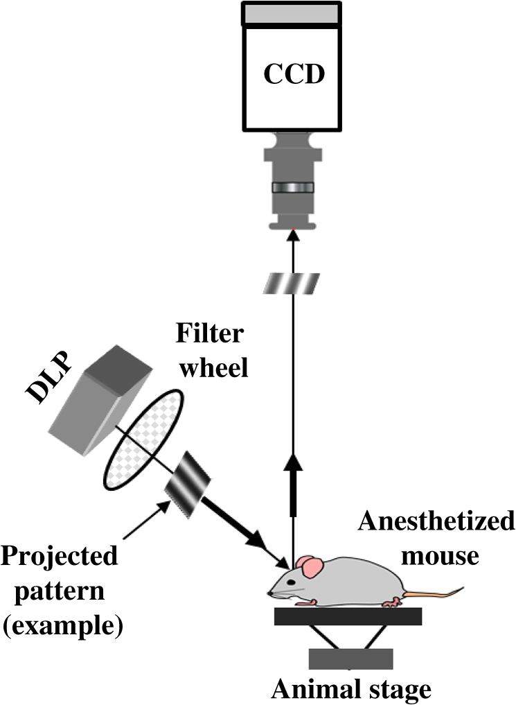
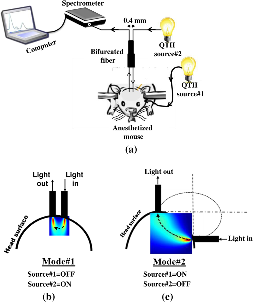
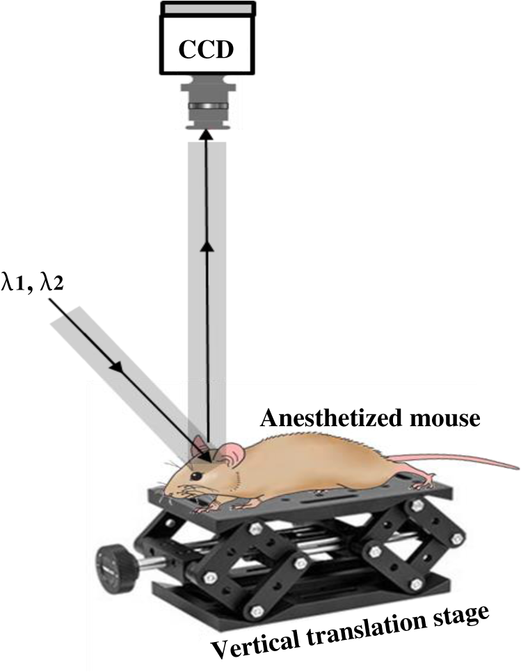
1.IntroductionThe last several decades have witnessed the development of numerous optical techniques for biomedical diagnosis and monitoring of therapy.1–3 These techniques offer several advantages over the traditional nonoptical methods, such as computed tomography, positron emission tomography, magnetic resonance imaging, and so on. Prominently, optical techniques are set apart by their simple structure, lower cost, and ease of handling. Furthermore, optical modalities are both portable and free from the adverse effects of ionizing radiation, enabling their use repeatedly at the patient’s bedside, for frequent or even continuous monitoring of patients’ vital parameters. All near-infrared (NIR, 650 to 1000 nm) optical imaging systems that monitor hemodynamic parameters of biological tissue such as hemoglobin concentration and oxygen saturation levels, as well as structural changes in tissue, obtain measurements indirectly from the tissue’s absorption and scattering coefficients of diffuse reflected (or transmitted) light.4–9 Thus, dynamic changes in the physiological properties of tissue can be detected via changes in these optical coefficients. Technically, the tissue is illuminated either by a laser or by a white light source, such as a light-emitting diode, resulting in diffusely reflected (or transmitted) light, which is captured by a camera or detector(s). Thus, an inverse model of light propagation relates the collected signal to optical properties of tissue to extract absorption and reduced scattering coefficients.10–14 Using a wavelength-dependent linear-square fit of absorption coefficient values and the Beer-Lambert law, the concentrations of individual chromophores (hemoglobin, lipids, water, and others) can be calculated,15,16 while structural variation of tissue can be derived from the scattering coefficients (amplitude and power) by Mie theory.17 The current array of studies demonstrates the use of three different optical systems as diagnostic assays to investigate the pathophysiological processes involved in focal traumatic brain injury (TBI). Normal brain function depends upon the delivery of oxygen, glucose, nutrients, and upon clearance of metabolism by-products.18 Following brain injury, both of these mechanisms are altered. Most importantly, there is a disruption in cellular respiration, leading to altered cellular and extracellular osmolarity, increased lactate levels and lowered extracellular pH, abnormal glutamate signaling (excitotoxicity), ATP depletion, and so on.19,20 In addition, increased intracranial pressure, brain herniation, inflammation, and vascular compression occur.21–24 Overall, these changes are reflected in hemodynamic and metabolic parameters, as well as in altered cellular morphology over time in brain tissue. The optical properties of the same can be quantified using the Beer-Lambert law and Mie scattering approximation. There are two major types of TBI: penetrating (direct impact, such as a bullet wound) and closed (indirect impact, such as that resulting from a car accident).25–27 The latter injury causes two types of brain damage: primary (skull fracture, contusions, hematomas, and nerve damage) as well as secondary (brain swelling, epilepsy, intracranial infection, raised intracranial pressure, and so on). Common to all head injuries are excitotoxicity and oxidative stress mechanisms, caused primarily by excessive glutamate neurotransmission, invoking a cascade of pathophysiological events leading to brain edema, increased intracranial pressure, and impaired cerebral perfusion (decreased blood flow), resulting eventually in neuronal cell death.28–30 The present research employed a model of a closed head injury (CHI) induced by a weight-drop apparatus, well-established to trigger a cascade of neurophysiological deficits and cell death.31,32 CHI is usually caused by blows to the head, which cause dynamic shifts of the brain within the skull, as in traffic accidents, falls, and assaults. In this type of trauma, the skull and dura mater remain intact, but oxygen delivery, metabolism, and the levels of glucose and other nutrients are severely altered, leading to neuronal damage.33 In the clinic, accurate monitoring of the dynamic changes in brain hemodynamics and metabolism following head trauma is invaluable for injury prognosis and for planning of optimal treatment. The three optical systems used in this work to quantify the changes in brain tissue chromophores, morphology, blood flow, and metabolism in the first critical hour of CHI in intact mice heads are NIR structured light illumination (a.k.a. spatially modulated illumination), orthogonal diffuse light spectroscopy, and dual-wavelength laser speckle imaging (DW-LSI). Each instrument array employs a different mode of operation and data analysis to derive brain tissue properties, as reviewed in Sec. 2. Section 3 reviews the experimental results and their interpretation in order to illustrate the effectiveness of these setups, with Sec. 4 concluding this review. 2.Methods and Materials2.1.Ethics StatementAnimal housing, care, and experimental procedures described below were reviewed and approved by the Institutional Animal Care and Use Committee of Ariel University, and was in compliance with the NIH/USDA guidelines for care and handling of laboratory animals. 2.2.Animal PreparationA total of 25 mice (imprinting control region mouse, weeks old, purchased from Harlan Laboratories, Jerusalem, Israel) were used in the research: 5 for the NIR structured light instrument and 10 for each of the other two optical instruments. The mice were housed in a research animal facility maintained at and relative humidity of , placed under a 12-h reverse light/dark cycle with free access to food and water. Each animal was intravenously anesthetized with a mixture of ketamine (), xylazine (), and saline (NaCl, 0.9%). The depth of anesthesia was sufficient to eliminate foot withdrawal to pinch, corneal reflex, or vibrissal movements. After the mouse was anesthetized, it was immobilized in an in-house-made head mount, scalp hair was carefully removed using a human hair removing lotion, and a sponge was inserted underneath the chin. Animals respired spontaneously, and their core body temperatures were monitored continuously during the experiment with rectal temperature probes (yellow springs instrument company) inserted into the rectum. Arterial oxygen saturation (), heart rate, and respiratory rate were monitored by oximeter (Nonin 8600) connected to the forelimb throughout the experiments. All mice were kept in their colony room until the day of the experiment. 2.3.Brain Injury ModelFor the induction of brain injury, we used the weight-drop technique in which a 50 gr cylindrical metallic rod is released from a height of above the mouse head along a metal tube positioned such that the weight strikes the mouse’s scalp between the anterior coronal suture (bregma) and posterior coronal suture (lambda). This rodent model of CHI closely mimics real-life focal head trauma and does not produce apparent structural damage to the brain.34 Baseline reflectance measurements were obtained prior to induction of injury, after which the mouse was removed and placed under the weight-drop device orthogonal to the point of impact. Thus, each mouse served as its own control, decreasing the number of animals required. Immediately after injury, the mouse was returned to the optical setup and the effects of injury were studied 1 h post-trauma. The animals remained anesthetized during the entire experiment and mice were culled in a chamber at experiment termination. Experiments were conducted successfully and no significant painful symptoms were observed. 2.4.Instruments DescriptionIn this section, we briefly describe the three optical setups used for obtaining optical properties and hemodynamics of brain tissue pre- and postinjury. Each instrument has its own operation and capabilities, substantially affecting its performance and resolution. 2.4.1.Spatially modulated illuminationSpatially modulated illumination features high spatiotemporal resolution and is able to control optical sampling depth (optical sectioning).35 Over recent decades, several studies have described the instrumentation of spatially modulated illumination and its use in noncontact and scan-free imaging in a variety of biomedical applications36–42 and in the clinic.43 Spatially modulated illumination is a multispectral wide-field imaging modality that utilizes NIR periodic illumination patterns with sinusoidal frequencies of up to to separately derive and spatially map the absolute values of the optical properties of tissue, i.e., absorption () and reduced light scattering () coefficients of turbid media. This separation (decoupling scattering from absorption) can be used to quantify the tissue’s chemical constituents (related to light absorption) and structural properties (related to light scattering). A schematic diagram of the system used in the present study is presented in Fig. 1. The main components of the system include a modified commercial digital light projector (PLUS, U5-112) based digital micromirrors device, filter wheel (Thorlabs, FW102C) placed before the projector, a CCD camera (Prosilica, GX1920, AVT), and computer station. The entire setup is controlled by MATLAB® software (MathWorks, Massachusetts). The wheel is equipped with six band-pass filters in the NIR region. At each wavelength, sinusoidal patterns are serially projected onto the head four times: three times with the same spatial frequency () with a phase shift of 120 deg between three adjacent patterns and one more illumination at zero spatial frequency () without phase shift (uniform wide-field illumination). These patterns are generated in the computer via MATLAB® software and are projected sequentially on the scalp. The goal of the projector modification is to obtain a small and adjustable illumination area with a stable, high-intensity light source in the NIR region. The diffusely reflected light is captured with a CCD camera, having a resolution of pixels (of ), mounted normal to the head surface, and saved in TIFF format for offline processing and analysis using MATLAB® software. CCD exposure time is automatically adjusted for each sampled wavelength during the calibration process. Image sets of each of the six wavelengths are then acquired at low and high spatial frequencies of 0 and , respectively, to determine the absorption and reduced scattering coefficients. While higher spatial frequency patterns are primarily sensitive to scattering changes but are insensitive to absorption, the lower spatial frequency patterns are more sensitive to changes in absorption but are insensitive to scattering.44,45 High spatial frequency is analogous to a small source–detector separation, while a large separation is equivalent to low spatial frequency. Therefore, minimum measurements of two spatial frequencies, low and high, can result in different sensitivities to absorption and scattering. Thus, sampling with more spatial frequencies and wavelengths will result in greater accuracy. By averaging each scattering image at each wavelength, the scattering spectra of brain tissue can be derived based on a simplified Mie scattering theory via the power law equation in the form , where is the scattering amplitude and sp is the scattering power.46,47 Analyzing the spectra of scattered light at all wavelengths by fitting the scattering values to a power law function, information regarding macroscopic cellular morphology can be retrieved throughout the scattering magnitude () and power (sp). In particular, sp (the slope of Mie scattering) is related to the mean size of the tissue scatterers (cell membrane, nuclei, lysosomes, mitochondria, and other organelles in the tissue) and defines spectral behavior of the reduced scattering coefficient, while is related to the density and distribution of scatterers. Usually, in the NIR region, ranged between 1.8 and . Specifically, the value and sign of sp is frequently used to differentiate tissue pathologies.48,49 Once the absorption coefficient spectra is known [] and combined with the wavelength-dependent molar extinction coefficients , metabolic properties () like perfusion, oxygenation, and chemical content (hemoglobin concentration, lipid, water, and so on) can be derived by applying the least-squares solution to the Beer-Lambert law, , as is commonly employed in tissue optics.50,51 As mentioned above, imaging is commenced before induction CHI to establish baseline chromophore concentrations and continued during and following experimental intervention. Prior to data analysis, the collected diffuse image is filtered to improve image quality. The calibration and validation of this technique were described at length in Ref. 52 regarding a flat homogenous tissue-mimicking phantom with known optical properties. 2.4.2.Orthogonal near-infrared spectroscopyThe schematic layout of the orthogonal spectroscopic setup is illustrated in Fig. 2(a). This configuration collected the diffuse reflected light at two designated distances from the light source in order to provide a quantitative assessment of the functional changes in sample tissue structure and composition. The system features two broadband light sources, a bifurcated fiber optic probe placed in direct contact with the scalp surface, a spectrometer, and computer station with control software. The optical fibers are connected to an mechanical stage translation for position control, and care was taken to ensure full contact between the probes and scalp surface throughout the experiments. Two broadband quartz-tungsten-halogen (QTH) lamp (IT, 9596-ER) were used to provide a smooth continuum and time-stable broadband spectral profile across the NIR region. The optical fiber connected to this light source was placed above the right ear. A fraction of the diffuse reflected light emanating from the head surface was delivered to a portable spectrometer (USB4000-VIS-NIR, Ocean Optics) with a spectral range of to 1000 nm by a bifurcated fiber mounted perpendicular to the scalp surface and hence orthogonal to the first light source fiber. Although the spectral range of the spectrometer is wide, wavelengths below 650 nm were not included in the data processing. The bifurcated fiber probe is composed of two branches: one branch is connected to the second white light source (HL-2000-FHSA-LL, Ocean Optics Inc.) and the other, for light collection, to the spectrometer. The receiver fiber collects the diffuse reflected light [] in two operation modes—mode 1 [Fig. 2(b), light source#1=OFF, light source#2=ON]: source–detector separation is [] and mode 2 [Fig. 2(c), light source#1=ON, light source#2=OFF]: []. Consequentially, measurements from these two modes of operation result in both different sensitivities to reduced scattering (mode 1) as well as absorption coefficients (mode 2), which in turn enable us to independently study the morphological conditions (via the power law) or brain tissue chromophore concentration (via Beer’s law). Thus, switching the illumination provided different spectroscopic sensitivity, such that mode 1 (single-fiber probe) can detect single scattered photons from a turbid media whose spectrum changes with size, shape, and refraction index of scatterers. Computer simulations of light propagation from source to the detector for each mode of operation are also presented in Figs. 2(b) and 2(c), respectively. It is worthwhile to emphasize that the depth sampling here can be tuned by merely positioning the ON/OFF switch, rather than by adjusting probe geometry as required by most diffuse reflectance spectroscopy systems.53–56 Also noteworthy is that once one of the light sources is operated (ON), the second source is automatically blocked (OFF) and vice versa. In this manner, we avoid any potential cross talk between the two modes. The measured NIR diffuse reflectance spectra underwent reflectance correction to compensate for the system’s spectral response, fibers attenuation, instrument drift, and for the detector’s own dark current. The calibration and validation of this technique was detailed previously, based on reference tissue-simulating phantom experiments with known optical properties.57 In contrast to the above structured illumination technique, we use here 500 wavelengths, which dramatically increase our spectral resolution and, therefore, the accuracy of the results. This is currently achieved at the expense of the field of vision imaged, since single-point measurements cannot provide spatial information. 2.4.3.Dual-wavelength laser speckle imagingDW-LSI combines laser speckle imaging and spectroscopic imaging into a single optical setup to probe cerebral hemodynamics and metabolism in real time.58 Laser speckle imaging detects dynamic blood flow changes within the medium by analyzing the random interference patterns resulting from scattered laser light with different path lengths.59,60 When a surface illuminated by coherent light (i.e., laser) is imaged by a camera, a random interference pattern known as a granule or speckle is formed.61 If the scattering particles, such as red blood cells, are in motion, a time-varying speckle pattern is generated at each pixel of the image.62 By analyzing the temporal and spatial intensity variations of this pattern, information about the movement can be estimated.63,64 The speckle variations have been said to be inversely related to the speed of the scattering elements. That is, with single shot imaging, a flow map with a large field of view and high spatiotemporal resolution is obtained. Various applications based on this camera-based imaging concept have been used to observe dynamic blood flow or tissue perfusion in the near-surface such as in skin,65,66 retina,67,68 optic nerve,69 mesentery,70 brain,71,72 stroke,73,74 hemorrhage,75 and during human neurosurgery.76 Figure 3 provides a schematic configuration of the DW-LSI setup. Compared to other related flow techniques, this scan-free full-field imaging technique is relatively low in cost, easy to implement and maintain, and operates at a high spatiotemporal resolution. Technically, two coherent beams from a diode laser operating at 530 and 660 nm, respectively, are switched by optical chopper such that only one wavelength is transmitted at any given time, preventing cross talk. We chose to work with a wavelength of 530 nm since this represents the isosbestic point at which oxy- and deoxyhemoglobin absorb light equally. Thus, the 530 nm laser obtains total hemoglobin concentration (THC), and changes in reflection at this wavelength are proportional to THC or cerebral blood volume (CBV) and cerebral blood flow (CBF), assuming that the concentration of red blood cells (hematocrit) remains constant ().77 The 660 nm laser was selected to differentiate between oxy- and deoxyhemoglobin based upon the gap between absorption coefficients of the two parameters ().1,78–80 Although there are other brain constituents, such as lipids, water, and so on, their absorption coefficients within those two wavelengths are several orders of magnitude smaller than the absorption coefficient for oxy- and deoxyhemoglobin (two dominant absorbers). Each of the laser beams is collimated and expanded by a lens system (not shown) into a uniform beam and then oblique illuminated the region of interest such that specular reflections do not affect the measurements. The diffuse reflectance image from the head at each wavelength is recorded by a 14-bit monochrome CCD camera (Guppy PRO F-031B, Allied Vision Technologies) equipped with a macro zoom lens (Computar, MLH10X, F5.6-32, Japan), positioned 16 cm above the head whose F-number () was set to meet the Nyquist criterion (speckle size camera pixel size) for flow imaging.81 Speckle size (second-order statistic) is dependent on the laser wavelength (), aperture size of the camera (), and the magnification (), given by .82 By controlling the of the lens, an optimal speckle size can be chosen. Camera integration time was set to 10 ms in order to optimize the contrast-to-noise ratio as well as sensitivity to flow changes.83 Imaging acquisition, synchronization, and data processing are achieved using in-house developed MATLAB® routines. Before data analysis, the collected raw diffuse images from 530 and 660 nm were saved in TIFF format and sorted using MATLAB® software based on differences in gray levels of each image. Next, these images were normalized to overcome the nonlinearity of the camera quantum efficiency at the above wavelengths, after which they were digitally filtered to remove periodic noise due to heart beat and respiration and to eliminate the high-frequency noise originating from the camera itself during recording. After data collection and preprocessing, a sliding-window algorithm ( pixel dimension) was applied to convert each 660 nm raw laser speckle image ( pixel dimension) to a speckle contrast image, , (first-order statistic) quantified by the ratio of the image’s standard deviation () to its mean gray-level intensity () over the small window.84,85 During experiments, 30 consecutive frames were averaged together into one speckle contrast image. Assuming Lorentzian velocity distribution, is inversely proportional to the blood flow velocity (motion of scattering particles), such that lower speed results in higher and vice versa.86–88 For instance, is close to unity if there is no movement within the medium. Concomitant to flow measurements, temporal changes in concentrations of the brain metabolism biomarkers oxyhemoglobin () and deoxyhemoglobin () can be extracted from the diffuse reflectance data by the Beer-Lambert method.89 Another indicator of cellular metabolism of interest to the neuroscience community is cytochrome-c-oxidase (CCO). The cerebral concentration of CCO is about an order of magnitude less than and Hbr, and is thus easily masked by these latter chromophores. One strategy to overcome this limitation is to use a series of wavelengths in order to increase signal-to-noise ratio and to decrease cross talk artifacts.90 In contrast to the two techniques mentioned in Secs. 2.4.1 and 2.4.2, here we use only two wavelengths emanating from coherent sources, which decrease our spectral resolution and accuracy. However, with this assay, we are able to map the blood flow with higher spatiotemporal resolution than previously achieved. For example, the blood flow monitoring with the widely used laser Doppler flowmetry (LDF) is highly localized, without spatial distribution information.91 On the other hand, speckle contrast imaging does not provide depth specificity () and flow velocity values in absolute units. In addition, since first- and second-order statistics are used, the estimation of speckle contrast is somewhat noisy, leading to reduced contrast resolution. 2.4.4.System comparisonsAs will be demonstrated in Sec. 3, while each method detects the same profile of changes in brain physiology parameters, each has its own advantages and disadvantages. Structured NIR illumination is a wide-field, noncontact imaging platform able to quantify and map separately optical properties as well as the concentration of various chromophores at the resolution of individual pixels. In addition, tomography (optical sectioning) can be achieved by changing the spatial frequency. However, the spectral and time resolutions are still limited. In addition, information on blood flow or tissue perfusion cannot be achieved directly. Furthermore, structured NIR is expensive in comparison to the other two setups. Orthogonal NIR spectroscopy uses hundreds of separate wavelengths, which increases the spectral resolution and the accuracy of results. It is able to separate the absorption and scattering effects simply, without using multiple sources and detectors or light propagation models in tissue. Information is obtained regarding different chromophore parameters from deep within tissue, not merely from the surface. Furthermore, this technique is low in cost in comparison to the other two setups. However, this technique cannot provide spatial information since it is a single-point measurement method, and thus does not enable mapping of blood flow. While the current setup requires contact with tissue, it can be modified using lenses to be a noncontact modality. DW-LSI is a wide-field, noncontact, and scan-free imaging platform capable of simultaneous mapping of changes in blood flow, hemodynamics, and metabolism using coherent light sources, with high spatiotemporal resolution. This technique requires no calibration and its data analysis is simple and straightforward. On the other hand, it provides insufficient information regarding the optical properties (absorption and scattering) and certain physiological parameters such as lipid and water concentrations. The technique’s penetration depth is also somewhat limited; deep tissue blood flow and oxygenation measurements are hard to get. 2.5.Statistical AnalysisThe experimental results are presented as mean ± standard error (), and two-way analysis of variance was performed to determine significant differences, with a value used as the significance cutoff. Calculations were carried out using MATLAB®’s Statistic Toolbox (MathWorks). It should be noted that although the head is a complex structure containing many tissue layers, in mice, these layers are very thin (skull , brain ), therefore, we consider the head as a homogenous medium. Hence, the results of the recovered properties represent the averaged values of a single volume. 3.Results and Discussion3.1.Study#1: Spatially Near-Infrared Modulated IlluminationFigure 4(a) shows bar graphs of the average and standard error (SE) of both chromophore concentrations and scattering properties, averaged along 1 h postinjury in comparison to preinjury, for five mice. CHI was found to have a significant impact on and following injury; both dropped during the observation period because of decrease in oxygen delivery to the brain and decreased blood supply to the injured zone. Moreover, this decrease reflects the acute effects of neurotrauma and the hemodynamic response during the early minutes of injury.92–95 In contrast, an increase in Hbr is seen, which may relate to increased capillary and venous blood stasis following injury. Assuming constant hematocrit (RBC concentration) levels, THC can serve as an indirect indicator of CBF. Reduced CBF reflects changes in energy demand and metabolism in the injured area, leading to disrupted oxygen balance and secondary injury in the brain. Reduced CBF is consistent with published data of alterations in CBF following TBI in both humans and animal models.96,97 This reduced flow is also supported by data provided by the third instrumentation setup (Sec. 3.3). In contrast to other hemodynamic parameters, tissue lipid levels do not change substantially during injury. In general, variation in lipid concentrations may indicate the dysregulation of lipid metabolism within brain cells. Altered lipid metabolism is believed to contribute to secondary brain injury, which occurs following traumatic brain injury.98,99 The changes in lipids following CHI are limited and will be the subject of our future research. Unfortunately, water concentration is not presented by the NIR structured system, due to the low quantum efficiency of the camera used at wavelength of 970 nm, which yielded a poor signal-to-noise ratio. Nonetheless, water level measurement is feasible utilizing a more highly powered camera. Apart from this, changes of up to 10% in scattering power (sp) from baseline were observed, attributed to cellular swelling and edema. In all presented parameters, no return to the baseline level was observed, emphasizing the critical condition of the brain during the acute postinjury phase. Figure 4(b) presents a typical map (normalized) of oxygen saturation and scattering power (the most significant parameters), demonstrating hemodynamics and tissue structure changes, respectively, preinjury and 1 h postinjury from a representative mouse experiment. The mean ± SE of entire images is outlined above each panel. The effects of injury on brain tissue are clearly visible in these maps. It should be noted that in the normalized scattering map, the increased pixel intensity reflects decreased sp value and vice versa. Averaging these maps reveals a decrease of 43 and 32% in tissue oxygen saturation and scattering power, respectively. These maps demonstrate the instrumentation setup’s capability to provide profound insight regarding spatial structural and hemodynamics variations of cerebral tissue following trauma. Overall, the changes we monitored reflect the pathophysiologic state of the brain following CHI (damaged blood vessels, altered CBF and physiology, neuronal cell death, and so on) and reveal the potential of this biomedical platform as an imaging tool to quantify changes in chromophore concentrations and morphologic variations over time. Fig. 4(a) Bar graph representing the average () hemodynamic and morphologic magnitude over 1 h postinjury. Each bar represents the average and standard error () of the mean. ; (paired -test). (b) Spatiotemporal maps illustrating distribution of the normalized brain tissue oxygenation (up) and scattering power (down), preinjury and 1 h postinjury. Each image map covers an area of , which corresponds to , and results in a spatial resolution of 0.015 mm/pixel. Color scale shows normalized changes. Changes of 43 and 32% in oxygenation and scattering power from baseline, respectively, are evident 1 h postinjury. Reduced indicates decreased oxygen delivery to the brain and failure of cellular respiration. Increase in normalized sp map, alternatively decrease in sp, implies an increase in average scattering particle size (mitochondria, other cytoplasmic organelles, cell nuclei, and so on)—cell swelling. 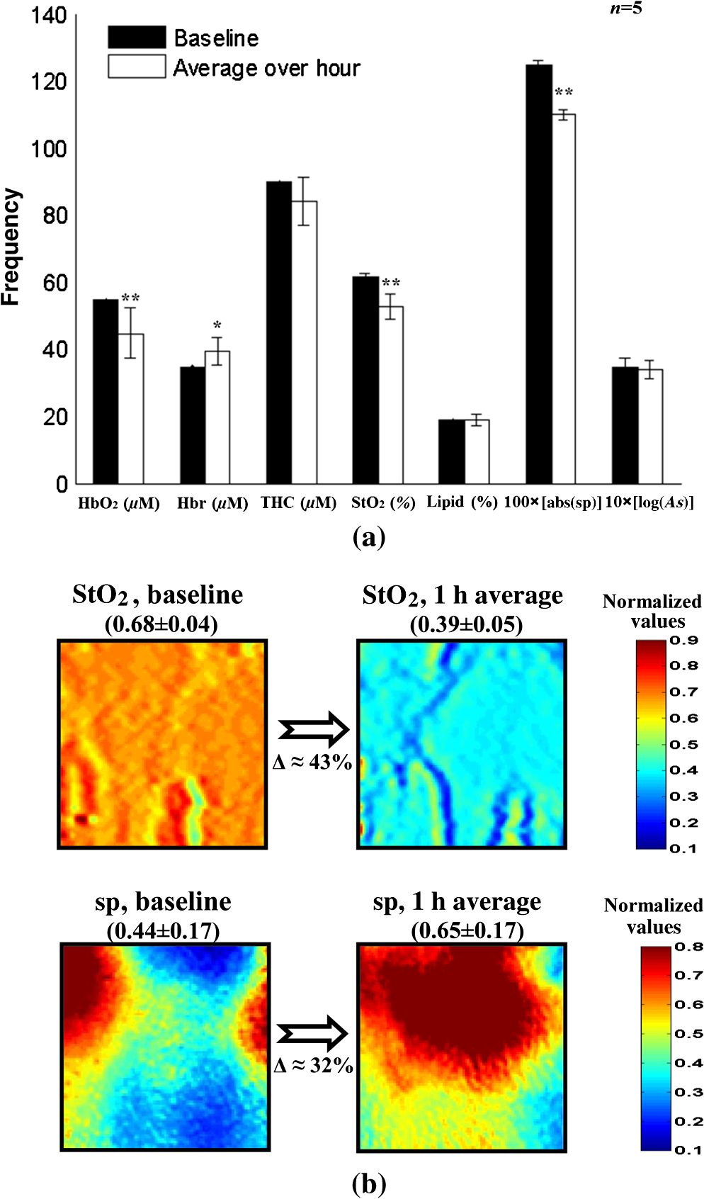 3.2.Study#2: Orthogonal SpectroscopyThe normalized reduced scattering spectra and absorption coefficients of a representative mouse pre- and postinjury as measured by both mode#1 and mode#2 of the spectroscopy system are demonstrated in Figs. 5(a) and 5(b), respectively. Variations in slope of the normalized scattering spectra over time postinjury appear prominently in Fig. 5(a), reflecting the changes in average particle size distribution (expansion and shrinkage). Specifically, the reduction in slope can be attributed to cellular and subcellular edema in response to injury, as supported by increased water levels in Fig. 5(c). The morphological changes are related to swelling of cellular and subcellular structures, mitochondrial dysfunction, and dendritic beading, all indicators of neuronal damage. Along the same line, variation in the absorption spectra relative to baseline [upper panel, Fig. 5(b)] highlights the changes in hemodynamics following injury. In the upper panel of Fig. 5(b), representing baseline measurements, no significant fluctuations over time in absorption are observed, reflecting measurement stability. A bar graph summarizing hemodynamic and morphological properties of 10 mice is presented in Fig. 5(c). Similar to Fig. 4(a), decreased , THC, and were observed postinjury, together with Hbr elevation by . Under decreased CBF (THC), brain cells undergo a series of pathophysiologic changes further complicated by the decreased oxygen supply, reflected in lowered , leading to secondary injury. Reduced indicates decreased oxygen delivery to the brain, encouraging anaerobic metabolism, yielding lactic acid buildup and energy failure (ATP depletion), which can lead to permanent brain damage, neurological disorders, reduced neuronal activity, or even death. Our findings of water content variations after injury agree with other studies.100–102 The increased water level we observed is corroborated by the decreased slope of reduced scattering [Fig. 5(a)], attributed to cellular swelling within brain structures. Water content variations after injury were also observed in Ref. 103 (p. 5411, Group 2, Table 2) using the dry/wet weight method. In this report, concentrations of were observed 1 h after injury. In our experiments, water content was observed. This slight discrepancy may be explained by the different setups and animal strains employed, or by variation in experimental conditions, although such discrepancies are considered minute in the biological context. Generally speaking, cerebral edema is swelling of the brain that occurs when free water escapes from within blood vessels in the brain into the brain tissue.104 It is divided into three categories: vasogenic edema (VE), cytotoxic edema, and interstitial edema.105 In all the three mentioned categories, the outer surface of the brain experiences an expansion that presses it against the inner surface of the skull followed by (1) displacement of the CSF layer surrounding the brain and (2) increased intracranial pressure.106,107 In our model of injury, VE is assumed to be occurring. Generally speaking, VE is the most common form of edema, and it is attributed to increased blood vessel capillary permeability.104,108 In VE, the normally tight cerebral endothelial cell junctions of capillaries are disrupted, and fluid exudes into the interstices between cells. From a tissue optics point of view, this will cause changes in cerebral optical properties and in hemodynamics. Specifically, brain swelling is accompanied by changes in the concentrations of oxyhemoglobin, deoxyhemoglobin, and water in brain tissue. These molecules absorb specific wavelengths of light, which alter the absorption properties of brain tissue. Along the same line, structural changes in the brain will introduce changes in (1) density and distribution of the scattering elements (cell membranes, organelle membrane, cellular nuclei, lysosomes, and other intracellular organelles, including the mitochondria), (2) refractive indices, and (3) average scatterer size, which can be studied through the scattering coefficient. Fig. 5(a) Representative normalized reduced scattering spectra from 650 to 1000 nm following injury as measured by mode#1 [Fig. 2(b)]. Variations in the slope after injury in contrast to baseline can be explained by the changes in the average scattering particle size, attributed to swelling and shrinkage of cellular and subcellular structures in response to injury. (b) Absorption coefficient spectra of the same from 650 to 1000 nm before (up) and after (down) injury as measured by mode#2 [Fig. 2(c)]. The spectral behavior of the absorption across 1 h in the upper panel indicates stability of measurements, while the variations shown in the lower panel indicate the changes in brain hemodynamics after injury. The absorption coefficient spectrum is related to the level of hemoglobin, lipid, water, and other absorbing agents, each with its unique extinction coefficients. (c) Bar graph demonstrates the average () hemodynamic and morphologic magnitude during 1 h postinjury. Each bar represents the mean and standard error () of the mean. , (paired -test). 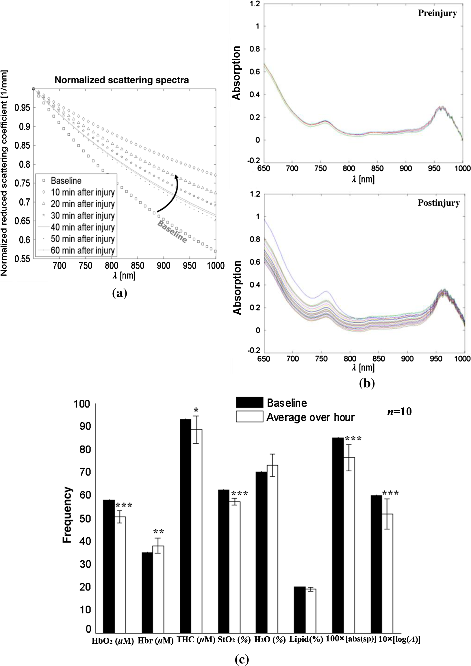 We wish to stress that in both systems, lipids are the only constituent measures that remained near their preinjury values. There is currently no consensus regarding alteration in lipid levels following brain injury. We will further examine in future studies the effect of focal TBI on lipids’ variation with larger animal populations. Altogether, these results reflect the pathophysiological state of the brain following trauma (damaged blood vessels, altered CBF and physiology, neuronal cell death, and so on) and strongly agree with other documented studies. The current findings reveal the potential of spectroscopy as a biomedical tool to quantify changes in chromophore concentrations and morphologic variations over time following brain injury. 3.3.Study#3: Dual Speckle ImagingThe relative hemodynamic and metabolic responses measured by the dual speckle approach, 1 h following injury are shown in Fig. 6(a), while the representative velocity distribution map, its corresponding pixel histogram profile, and three-dimensional representation, at specific points of time before (upper panels) and after (lower panels) injury are presented in Fig. 6(b), highlighting reduction in blood flow and metabolism at the onset of injury. In the maps, higher pixel values represent higher CBF velocity, which is inversely proportional to . Figure 6(a) displays clearly increased Hbr levels, alongside decreased , reflecting postinjury hypoxia as detected by the two previous systems. Elevated Hbr levels suggest the development of secondary brain damage stemming from ischemia, a common occurrence postinjury.109–112 The decrease in flow leads to disruption in oxygen balance, resulting in extracellular ion concentration irregularities, increased lactate levels, decreased extracellular pH, and abnormal accumulation of glutamate. Studies of CBF in severely head-injured patients show that altered CBF is related to poor clinical outcome.113 Decreased blood flow following injury was also observed in the raw reflectance images obtained at 530 nm (data not shown). The combined real-time monitoring of blood flow together with hemoglobin oxygenation provides insight to brain metabolism activity. Taken together, the hemodynamics and metabolism data hold clinical value for monitoring brain injury. The reduced oxygen metabolism is supported by the decreased cerebral metabolic rate of oxygen (), suggesting mitochondrial dysfunction and reduced oxygen consumption following injury. is proportional to the fractional changes in CBF, multiplied by that of Hbr, divided by that of THC.114 measures the difference between the rates at which oxygen flows in and out of a region of investigation. Studies have shown decreased postinjury to indicate reduced electrocortical activity, such that may serve as a biomarker of cerebral ischemia.115 In Fig. 6(b), each flow map covers an area of , corresponding to , resulting in an average spatial resolution of . As shown, decreasing map contrast indicates decreased blood flow over time. In addition, the histogram distribution indicates that pre- and postinjury states each possess a characteristic peak value and distribution, which may also serve as biomarkers of the brain’s pathophysiological state. By converting the flow maps into histogram distributions or three-dimensional representations during injury progression, additional insight to localized changes in the brain can be obtained on a pixel level. To validate the monitoring of CBF by dual speckle imaging, parallel measurements were taken with LDF (Periflux, ), which confirmed the reduced CBF following injury shown in Fig. 6(c). As demonstrated, CBF dropped by more than 13%, indicating decreased oxygen delivery to the brain accompanied by decreased cerebral perfusion, resulting in failure of autoregulation mechanisms and a further sustained decrease in CBF over time. In the final measurement point, a simple model of hypoxic ischemia (following euthanasia) was obtained, which causes a further decrease in an already limited blood supply leading to permanent neuronal damage and finally death. Two major findings that can be summarized from the above findings are that acute brain injury (1) modified the hemodynamic response and (2) induced significant changes in blood flow and metabolism. Overall, the three instruments detected variations in chromophore concentrations and brain metabolism following head injury in strong agreement with that known from other methods, highlighting the effectiveness of these approaches for intrinsic signal imaging and spectroscopy. Fig. 6(a) Magnitude changes in oxy- and deoxyhemoglobin, CBF, and cerebral metabolic rate during 1 h postinjury of all experiments (, average ± SE of the mean). (b) Representative flow distribution map, profiling blood flow along the horizontal dashed line, with corresponding flow histogram, and three-dimensional plot of flow map before (top) and after (bottom) injury. Each contrast map covers an area of , corresponding to , resulting in an average spatial resolution of . The vertical axis in each histogram reflects the number of counts in each bin and the solid curve in the histogram is a Gaussian fit with appropriate mean and standard deviation. Statistically significant differences highlight the impact of injury upon CBF. H, high flow; L, low flow. (c) Flow measured by LDF (Periflux) at three time points: baseline, 1 h postinjury, and 10 min after euthanasia ( for each bar). Each data point is presented as mean ± SE (); , , (paired -test). 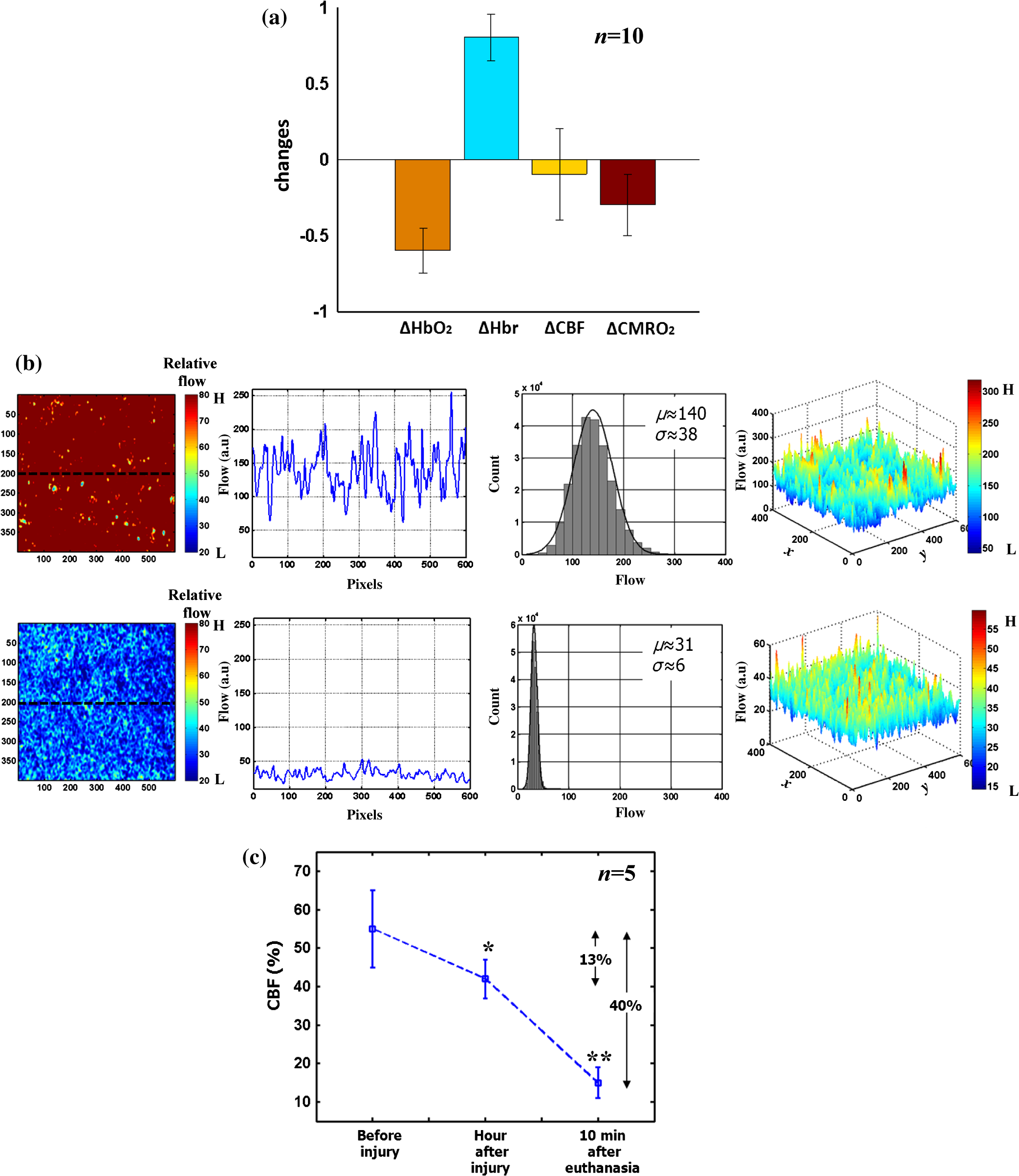 4.ConclusionIn the above findings, three different optical apparatuses—spatially modulated NIR illumination, orthogonal diffuse light spectroscopy, and DW-LSI—successfully assessed changes in the brain’s physiological parameters during the first critical hour following focal traumatic brain injury. Despite their differing modes of operation, each method detected the same profile of changes in a battery of brain physiology parameters, including decreased hemoglobin oxygen saturation level, CBF and rate of cellular metabolism, as well as changes in brain structural features. These results accurately reflect the pathophysiology of the brain following trauma, as known from a range of conventional methods. Taken together, this study demonstrates the great potential of these systems as noninvasive, quantitative tools for monitoring brain hemodynamics and metabolism following injury at the bedside or in the field. Since each of the three systems possesses its own unique benefits and limitations, we suggest future study of a multimodal approach combining complementary imaging methods for their further optimization. Moreover, the implementation of longer wavelengths in the spectral range of 1000 to 2000 nm, known as short-wave infrared (SWIR),116 will be considered in this proposed combined system. This region holds an important advantage for spectroscopy and imaging purposes: within this range, scattering is attenuated monotonically, leading to increased transparency of photons within the tissue and hence improved penetration depth.117,118 In addition, SWIR includes more absorption peaks, thereby adding additional information and hence improved sensitivity for various chromophores such as proteins, water, collagen, lipids, and so on.116,119,120 ReferencesD. A. Boas, C. Pitris and N. Ramanujam, Handbook of Biomedical Optics, CRC Press, Florida
(2011). Google Scholar
J. G. Fujimoto and D. L. Farkas, Biomedical Optical Imaging, Oxford University Press, Oxford; New York
(2009). Google Scholar
I. J. Bigio and S. Fantini, Quantitative Biomedical Optics: Theory, Methods, and Applications, Cambridge University Press, United Kingdom
(2016). Google Scholar
L. V. Wang and H. I. Wu, Biomedical Optics: Principles and Imaging, John Wiley & Sons, Inc., Hoboken, New Jersey
(2007). Google Scholar
V. V. Tuchin, Handbook of Optical Biomedical Diagnostics, SPIE Press, Bellingham, Washington
(2002). Google Scholar
M. A. Yaseen et al.,
“Multimodal optical imaging system for in vivo investigation of cerebral oxygen delivery and energy metabolism,”
Biomed. Opt. Express, 6
(12), 4994
–5007
(2015). http://dx.doi.org/10.1364/BOE.6.004994 Google Scholar
Y. Jia et al.,
“In vivo optical imaging of revascularization after brain trauma in mice,”
Microvasc. Res., 81
(1), 73
–80
(2011). http://dx.doi.org/10.1016/j.mvr.2010.11.003 Google Scholar
K. Yoshida et al.,
“Multispectral imaging of absorption and scattering properties of in vivo exposed rat brain using a digital red-green-blue camera,”
J. Biomed. Opt., 20
(5), 051026
(2015). http://dx.doi.org/10.1117/1.JBO.20.5.051026 Google Scholar
H. Cen and R. Lu,
“Optimization of the hyperspectral imaging-based spatially-resolved system for measuring the optical properties of biological materials,”
Opt. Express, 18
(16), 17412
–17432
(2010). http://dx.doi.org/10.1364/OE.18.017412 Google Scholar
K. W. Calabro and I. J. Bigio,
“Influence of the phase function in generalized diffuse reflectance models: review of current formalisms and novel observations,”
J. Biomed. Opt., 19
(7), 075005
(2014). http://dx.doi.org/10.1117/1.JBO.19.7.075005 Google Scholar
M. Sharma et al.,
“Verification of a two-layer inverse Monte Carlo absorption model using multiple source-detector separation diffuse reflectance spectroscopy,”
Biomed. Opt. Express, 5
(1), 40
–53
(2014). http://dx.doi.org/10.1364/BOE.5.000040 Google Scholar
R. Watté et al.,
“Metamodeling approach for efficient estimation of optical properties of turbid media from spatially resolved diffuse reflectance measurements,”
Opt. Express, 21
(26), 32630
–32642
(2013). http://dx.doi.org/10.1364/OE.21.032630 Google Scholar
A. Kim et al.,
“A fiberoptic reflectance probe with multiple source-collector separations to increase the dynamic range of derived tissue optical absorption and scattering coefficients,”
Opt. Express, 18
(6), 5580
–5594
(2010). http://dx.doi.org/10.1364/OE.18.005580 Google Scholar
M-W. Lee et al.,
“A linear gradient line source facilitates the use of diffusion models with high order approximation for efficient, accurate turbid sample optical properties recovery,”
Biomed. Opt. Express, 5
(10), 3628
–3639
(2014). http://dx.doi.org/10.1364/BOE.5.003628 Google Scholar
G. Strangman, M. A. Franceschini and D. A. Boas,
“Factors affecting the accuracy of near-infrared spectroscopy concentration calculations for focal changes in oxygenation parameters,”
Neuroimage, 18
(4), 865
–879
(2003). http://dx.doi.org/10.1016/S1053-8119(03)00021-1 Google Scholar
H. Liu et al.,
“Noninvasive investigation of blood oxygenation dynamics of tumors by near-infrared spectroscopy,”
Appl. Opt., 39
(28), 5231
–5243
(2000). http://dx.doi.org/10.1364/AO.39.005231 Google Scholar
C. Lau et al.,
“Re-evaluation of model-based light-scattering spectroscopy for tissue spectroscopy,”
J. Biomed. Opt., 14
(2), 024031
(2009). http://dx.doi.org/10.1117/1.3116708 Google Scholar
M. F. Bear, B. W. Connors and M. A. Paradiso, Neuroscience: Exploring the Brain, Williams & Wilkins, Baltimore, Maryland
(1996). Google Scholar
A. Zauner et al.,
“Brain oxygenation and energy metabolism: part I—biological function and pathophysiology,”
Neurosurgery, 51
(2), 289
–301
(2002). Google Scholar
S. H. Haddad and Y. M. Arabi,
“Critical care management of severe traumatic brain injury in adults,”
Scand. J. Trauma Resusc. Emerg. Med., 20
(12), 1
–15
(2012). http://dx.doi.org/10.1186/1757-7241-20-12 Google Scholar
P. Bouzat et al.,
“Beyond intracranial pressure: optimization of cerebral blood flow, oxygen, and substrate delivery after traumatic brain injury,”
Ann. Intensive Care, 3
(1), 23
(2013). http://dx.doi.org/10.1186/2110-5820-3-23 Google Scholar
A. Guha,
“Management of traumatic brain injury: some current evidence and applications,”
Postgrad. Med. J., 80
(949), 650
–653
(2004). http://dx.doi.org/10.1136/pgmj.2004.019570 Google Scholar
T. Woodcock and M. C. Morganti-Kossmann,
“The role of markers of inflammation in traumatic brain injury,”
Front. Neurol., 4
(18), 1
–18
(2013). http://dx.doi.org/10.3389/fneur.2013.00018. eCollection 2013 Google Scholar
S. I. Stiver, A. D. Gean and G. T. Manley,
“Survival with good outcome after cerebral herniation and Duret hemorrhage caused by traumatic brain injury,”
J. Neurosurg., 110
(6), 1242
–1246
(2009). http://dx.doi.org/10.3171/2008.8.JNS08314 Google Scholar
J. H. Adams, D. I. Graham and T. A. Gennarelli,
“Head injury in man and experimental animals: neuropathology,”
Acta Neurochir. Suppl., 32 15
–30
(1983). http://dx.doi.org/10.1007/978-3-7091-4147-2 Google Scholar
A. I. Maas, N. Stocchetti and R. Bullock,
“Moderate and severe traumatic brain injury in adults,”
Lancet Neurol., 7
(8), 728
–741
(2008). http://dx.doi.org/10.1016/S1474-4422(08)70164-9 Google Scholar
J. A. Langlois, W. Rutland-Brown and M. M. Wald,
“The epidemiology and impact of traumatic brain injury: a brief overview,”
J. Head Trauma Rehabil., 21
(5), 375
–378
(2006). http://dx.doi.org/10.1097/00001199-200609000-00001 Google Scholar
C. O. de Oliveira, N. Ikuta and A. Regner,
“Outcome biomarkers following severe traumatic brain injury,”
Rev. Bras. Ter. Intensiva, 20
(4), 411
–421
(2008). http://dx.doi.org/10.1590/S0103-507X2008000400015 Google Scholar
T. K. McIntosh et al.,
“Neuropathological sequelae of traumatic brain injury: relationship to neurochemical and biomechanical mechanisms,”
Lab. Invest., 74
(2), 315
–342
(1996). Google Scholar
J. H. Yi and A. S. Hazell,
“Excitotoxic mechanisms and the role of astrocytic glutamate transporters in traumatic brain injury,”
Neurochem. Int., 48
(5), 394
–403
(2006). http://dx.doi.org/10.1016/j.neuint.2005.12.001 Google Scholar
R. G. Grossman, Neurobehavioral Consequences of Closed Head Injury, Oxford University Press, New York
(1990). Google Scholar
R. L. Rodnitzky and M. Meier,
“Neurobehavioral consequences of closed head injury,”
Arch. Neurol., 39
(10), 675
–676
(1982). http://dx.doi.org/10.1001/archneur.1982.00510220073030 Google Scholar
J. T. E. Richardson, Clinical and Neuropsychological Aspects of Closed Head Injury, 2nd ed.Psychology Press, Philadelphia
(2002). Google Scholar
Y. Xiong, A. Mahmood and M. Chopp,
“Animal models of traumatic brain injury,”
Nat. Rev. Neurosci., 14
(2), 128
–142
(2013). http://dx.doi.org/10.1038/nrn3407 Google Scholar
D. J. Cuccia et al.,
“Modulated imaging: quantitative analysis and tomography of turbid media in the spatial-frequency domain,”
Opt. Lett., 30
(11), 1354
–1356
(2005). http://dx.doi.org/10.1364/OL.30.001354 Google Scholar
D. Abookasis et al.,
“Imaging cortical absorption, scattering, and hemodynamic response during ischemic stroke using spatially modulated near-infrared illumination,”
J. Biomed. Opt., 14
(2), 024033
(2009). http://dx.doi.org/10.1117/1.3116709 Google Scholar
D. Abookasis et al.,
“Using NIR spatial illumination for detection and mapping chromophores changes during cerebral edema,”
Proc. SPIE, 6842 68422U
(2008). http://dx.doi.org/10.1117/12.760516 Google Scholar
A. J. Lin et al.,
“Spatial frequency domain imaging of intrinsic optical property contrast in a mouse model of alzheimer’s disease,”
Ann. Biomed. Eng., 39
(4), 1349
–1357
(2011). http://dx.doi.org/10.1007/s10439-011-0269-6 Google Scholar
K. P. Nadeau et al.,
“Quantitative assessment of renal arterial occlusion in a porcine model using spatial frequency domain imaging,”
Opt. Lett., 38
(18), 3566
–3569
(2013). http://dx.doi.org/10.1364/OL.38.003566 Google Scholar
D. J. Rohrbach et al.,
“Characterization of nonmelanoma skin cancer for light therapy using spatial frequency domain imaging,”
Biomed. Opt. Express, 6
(5), 1761
–1766
(2015). http://dx.doi.org/10.1364/BOE.6.001761 Google Scholar
A. M. Laughney et al.,
“System analysis of spatial frequency domain imaging for quantitative mapping of surgically resected breast tissues,”
J. Biomed. Opt., 18
(3), 036012
(2013). http://dx.doi.org/10.1117/1.JBO.18.3.036012 Google Scholar
R. P. Singh-Moon et al.,
“Spatial mapping of drug delivery to brain tissue using hyperspectral spatial frequency-domain imaging,”
J. Biomed. Opt., 19
(9), 096003
(2014). http://dx.doi.org/10.1117/1.JBO.19.9.096003 Google Scholar
S. Gioux et al.,
“First-in-human pilot study of a spatial frequency domain oxygenation imaging system,”
J. Biomed. Opt., 16
(8), 086015
(2011). http://dx.doi.org/10.1117/1.3614566 Google Scholar
D. J. Cuccia et al.,
“Quantitation and mapping of tissue optical properties using modulated imaging,”
J. Biomed. Opt., 14
(2), 024012
(2009). http://dx.doi.org/10.1117/1.3088140 Google Scholar
T. D. O’sullivan et al.,
“Diffuse optical imaging using spatially and temporally modulated light,”
J. Biomed. Opt., 17
(7), 071311
(2012). http://dx.doi.org/10.1117/1.JBO.17.7.071311 Google Scholar
R. Graaff et al.,
“Reduced light-scattering properties for mixtures of spherical particles: a simple approximation derived from Mie calculations,”
Appl. Opt., 31
(10), 1370
–1376
(1992). http://dx.doi.org/10.1364/AO.31.001370 Google Scholar
J. R. Mourant et al.,
“Mechanisms of light scattering from biological cells relevant to noninvasive optical-tissue diagnostics,”
Appl. Opt., 37
(16), 3586
–3593
(1998). http://dx.doi.org/10.1364/AO.37.003586 Google Scholar
V. Tuchin, Tissue Optics: Light Scattering Methods and Instruments for Medical Diagnosis, 2nd ed.SPIE Press, Bellingham, Washington
(2007). Google Scholar
A. M. Laughney et al.,
“Scatter spectroscopic imaging distinguishes between breast pathologies in tissues relevant to surgical margin assessment,”
Clin. Cancer Res., 18
(22), 6315
–6325
(2012). http://dx.doi.org/10.1158/1078-0432.CCR-12-0136 Google Scholar
R. V. Maikala,
“Modified Beer’s Law—historical perspectives and relevance in near-infrared monitoring of optical properties of human tissue,”
J. Ind. Ergon., 40 125
–134
(2010). http://dx.doi.org/10.1016/j.ergon.2009.02.011 Google Scholar
I. Nishidate et al.,
“Noninvasive spectral imaging of skin chromophores based on multiple regression analysis aided by Monte Carlo simulation,”
Opt. Lett., 36
(16), 3239
–3241
(2011). http://dx.doi.org/10.1364/OL.36.003239 Google Scholar
D. Abookasis, B. Volkov and M. S. Mathews,
“Closed head injury-induced changes in brain pathophysiology assessed with near-infrared structured illumination in a mouse model,”
J. Biomed. Opt., 18
(11), 116007
(2013). http://dx.doi.org/10.1117/1.JBO.18.11.116007 Google Scholar
K. Vishwanath et al.,
“Portable, fiber-based, diffuse reflection spectroscopy (DRS) systems for estimating tissue optical properties,”
Appl. Spectrosc., 62
(2), 206
–215
(2011). http://dx.doi.org/10.1366/10-06052 Google Scholar
R. J. Mallia et al.,
“Diffuse reflection spectroscopy: an alternative to autofluorescence spectroscopy in tongue cancer detection,”
Appl. Spectrosc., 64
(4), 409
–418
(2010). http://dx.doi.org/10.1366/000370210791114347 Google Scholar
F. Koenig et al.,
“Spectroscopic measurement of diffuse reflectance for enhanced detection of bladder carcinoma,”
Urology, 51
(2), 342
–345
(1998). http://dx.doi.org/10.1016/S0090-4295(97)00612-2 Google Scholar
G. Zonios et al.,
“Diffuse reflectance spectroscopy of human adenomatous colon polyps in vivo,”
Appl. Opt., 38
(31), 6628
–6637
(1999). http://dx.doi.org/10.1364/AO.38.006628 Google Scholar
A. Shochat and D. Abookasis,
“Differential effects of early postinjury treatment with neuroprotective drugs in a mouse model using diffuse reflectance spectroscopy,”
Neurophotonics, 2
(1), 015001
(2015). http://dx.doi.org/10.1117/1.NPh.2.1.015001 Google Scholar
A. K. Dunn et al.,
“Simultaneous imaging of total cerebral hemoglobin concentration, oxygenation, and blood flow during functional activation,”
Opt. Lett., 28
(1), 28
–30
(2003). http://dx.doi.org/10.1364/OL.28.000028 Google Scholar
A. Fercher and J. Briers,
“Flow visualization by means of single exposure speckle photography,”
Opt. Commun., 37
(5), 326
–330
(1981). http://dx.doi.org/10.1016/0030-4018(81)90428-4 Google Scholar
J. D. Briers and S. Webster,
“Laser speckle contrast analysis (LASCA): a nonscanning, full-field technique for monitoring capillary blood flow,”
J. Biomed. Opt., 1
(2), 174
–179
(1996). http://dx.doi.org/10.1117/12.231359 Google Scholar
J. D. Briers,
“Laser Doppler, speckle and related techniques for blood perfusion mapping and imaging,”
Physiol. Meas., 22
(4), R35
–R66
(2001). http://dx.doi.org/10.1088/0967-3334/22/4/201 Google Scholar
P. Miao et al.,
“High resolution cerebral blood flow imaging by registered laser speckle contrast analysis,”
IEEE Trans. Biomed. Eng., 57
(5), 1152
–1157
(2010). http://dx.doi.org/10.1109/TBME.2009.2037434 Google Scholar
P. Miao et al.,
“Entropy analysis reveals a simple linear relation between laser speckle and blood flow,”
Opt. Lett., 39
(13), 3907
–3910
(2014). http://dx.doi.org/10.1364/OL.39.003907 Google Scholar
B. Choi et al.,
“Linear response range characterization and in vivo application of laser speckle imaging of blood flow dynamics,”
J. Biomed. Opt., 11
(4), 041129
(2006). http://dx.doi.org/10.1117/1.2341196 Google Scholar
B. Choi, N. M. Kang and J. S. Nelson,
“Laser speckle imaging for monitoring blood flow dynamics in the in vivo rodent dorsal skin fold model,”
Microvasc. Res., 68
(2), 143
–146
(2004). http://dx.doi.org/10.1016/j.mvr.2004.04.003 Google Scholar
A. Humeau-Heurtiera et al.,
“Skin perfusion evaluation between laser speckle contrast imaging and laser Doppler flowmetry,”
Opt. Commun., 291
(2013), 482
–487
(2013). http://dx.doi.org/10.1016/j.optcom.2012.11.054 Google Scholar
H. Cheng and T. Q. Duong,
“Simplified laser-speckle-imaging analysis method and its application to retinal blood flow imaging,”
Opt. Lett., 32
(15), 2188
–2190
(2007). http://dx.doi.org/10.1364/OL.32.002188 Google Scholar
A. Ponticorvo et al.,
“Laser speckle contrast imaging of blood flow in rat retinas using an endoscope,”
J. Biomed Opt., 18
(9), 090501
(2013). http://dx.doi.org/10.1117/1.JBO.18.9.090501 Google Scholar
L. Wang et al.,
“Anterior and posterior optic nerve head blood flow in nonhuman primate experimental glaucoma model measured by laser speckle imaging technique and microsphere method,”
Invest. Ophthalmol. Vis. Sci., 53
(13), 8303
–8309
(2012). http://dx.doi.org/10.1167/iovs.12-10911 Google Scholar
H. Cheng et al.,
“Efficient characterization of regional mesenteric blood flow by use of laser speckle imaging,”
Appl. Opt., 42
(28), 5759
–5764
(2003). http://dx.doi.org/10.1364/AO.42.005759 Google Scholar
P. Li et al.,
“Imaging cerebral blood flow through the intact rat skull with temporal laser speckle imaging,”
Opt. Lett., 31
(12), 1824
–1826
(2006). http://dx.doi.org/10.1364/OL.31.001824 Google Scholar
C. Wu et al.,
“A hybrid de-noising method on LASCA images of blood vessels,”
J. Signal Inf. Process., 3
(1), 92
–97
(2012). http://dx.doi.org/10.4236/jsip.2012.31012 Google Scholar
G. A. Armitage et al.,
“Laser speckle contrast imaging of collateral blood flow during acute ischemic stroke,”
J. Cereb. Blood Flow Metab., 30
(8), 1432
–1436
(2010). http://dx.doi.org/10.1038/jcbfm.2010.73 Google Scholar
H. Levy, D. Ringuette and O. Levi,
“Rapid monitoring of cerebral ischemia dynamics using laser-based optical imaging of blood oxygenation and flow,”
Biomed. Opt. Express, 3
(4), 777
–791
(2012). http://dx.doi.org/10.1364/BOE.3.000777 Google Scholar
A. N. Pavlov et al.,
“Hidden stage of intracranial hemorrhage in newborn rats studied with laser speckle contrast imaging and wavelets,”
J. Innov. Opt. Health Sci., 8
(5), 1550041
(2015). http://dx.doi.org/10.1142/S1793545815500418 Google Scholar
A. B. Parthasarathy et al.,
“Laser speckle contrast imaging of cerebral blood flow in humans during neurosurgery: a pilot clinical study,”
J. Biomed. Opt., 15
(6), 066030
(2010). http://dx.doi.org/10.1117/1.3526368 Google Scholar
R. L. Grubb et al.,
“The effects of changes in on cerebral blood volume, blood flow, and vascular mean transit time,”
Stroke, 5
(5), 630
–639
(1974). http://dx.doi.org/10.1161/01.STR.5.5.630 Google Scholar
S. Prahl,
“Hemoglobin absorption coefficient,”
(1999) http://omlc.ogi.edu/spectra/hemoglobin/index.html ( January 2016). Google Scholar
A. Deutsch et al.,
“Real time evaluation of tissue vitality by monitoring of microcirculatory blood flow, , and mitochondrial NADH redox state,”
Proc. SPIE, 5317 116
–127
(2004). http://dx.doi.org/10.1117/12.528601 Google Scholar
R. Nachabé et al.,
“Estimation of biological chromophores using diffuse optical spectroscopy: benefit of extending the UV-VIS wavelength range to include 1000 to 1600 nm,”
Biomed. Opt. Express, 1
(5), 1432
–1442
(2010). http://dx.doi.org/10.1364/BOE.1.001432 Google Scholar
D. Briers et al.,
“Laser speckle contrast imaging: theoretical and practical limitations,”
J. Biomed. Opt., 18
(6), 066018
(2013). http://dx.doi.org/10.1117/1.JBO.18.6.066018 Google Scholar
D. A. Boas and A. K. Dunn,
“Laser speckle contrast imaging in biomedical optics,”
J. Biomed. Opt., 15
(1), 011109
(2010). http://dx.doi.org/10.1117/1.3285504 Google Scholar
S. Yuan et al.,
“Determination of optimal exposure time for imaging of blood flow changes with laser speckle contrast imaging,”
Appl. Opt., 44
(10), 1823
–1830
(2005). http://dx.doi.org/10.1364/AO.44.001823 Google Scholar
D. D. Duncan, S. J. Kirkpatrick and R. K. Wang,
“Statistics of local speckle contrast,”
JOSA A, 25
(1), 9
–15
(2008). http://dx.doi.org/10.1364/JOSAA.25.000009 Google Scholar
P. Zakharov et al.,
“Dynamic laser speckle imaging of cerebral blood flow,”
Opt. Express, 17
(16), 13904
–13917
(2009). http://dx.doi.org/10.1364/OE.17.013904 Google Scholar
O. Yang and B. Choi,
“Laser speckle imaging using a consumer-grade color camera,”
Opt. Lett., 37
(19), 3957
–3959
(2012). http://dx.doi.org/10.1364/OL.37.003957 Google Scholar
J. K. Meisner et al.,
“Trans-illuminated laser speckle imaging of collateral artery blood flow in ischemic mouse hindlimb,”
J. Biomed. Opt., 18
(9), 096011
(2013). http://dx.doi.org/10.1117/1.JBO.18.9.096011 Google Scholar
R. Bi, J. Dong and K. Lee,
“Deep tissue flowmetry based on diffuse speckle contrast analysis,”
Opt. Lett., 38
(9), 1401
–1403
(2013). http://dx.doi.org/10.1364/OL.38.001401 Google Scholar
Z. Luo et al.,
“Simultaneous imaging of cortical hemodynamics and blood oxygenation change during cerebral ischemia using dual-wavelength laser speckle contrast imaging,”
Opt. Lett., 34
(9), 1480
–1482
(2009). http://dx.doi.org/10.1364/OL.34.001480 Google Scholar
D. Arifler et al.,
“Optimal wavelength combinations for near-infrared spectroscopic monitoring of changes in brain tissue hemoglobin and cytochrome c oxidase concentrations,”
Biomed. Opt. Express, 6
(3), 933
–947
(2015). http://dx.doi.org/10.1364/BOE.6.000933 Google Scholar
J. D. Briers,
“Laser Doppler, speckle and related techniques for blood perfusion mapping and imaging,”
Physiol. Meas., 22
(4), R35
–R66
(2001). http://dx.doi.org/10.1088/0967-3334/22/4/201 Google Scholar
A. T. Minassian et al.,
“Correlation between cerebral oxygen saturation measured by near-infrared spectroscopy and jugular oxygen saturation in patients with severe closed head injury,”
Anesthesiology, 91
(4), 985
–990
(1999). http://dx.doi.org/10.1097/00000542-199910000-00018 Google Scholar
E. Maloney-Wilensky et al.,
“Brain tissue oxygen and outcome after severe traumatic brain injury: a systematic review,”
Crit. Care Med., 37
(6), 2057
–2063
(2009). http://dx.doi.org/10.1097/CCM.0b013e3181a009f8 Google Scholar
D. A. Boas and M. A. Franceschini,
“Haemoglobin oxygen saturation as a biomarker: the problem and a solution,”
Philos. Trans. A Math. Phys. Eng. Sci., 369
(1955), 4407
–4424
(2011). http://dx.doi.org/10.1098/rsta.2011.0250 Google Scholar
R. Shafer, A. Brown and C. Taylor,
“Correlation between cerebral blood flow and oxygen saturation in patients with subarachnoid hemorrhage and traumatic brain injury,”
J. Neurointerv. Surg., 3
(4), 395
–398
(2011). http://dx.doi.org/10.1136/jnis.2010.004184 Google Scholar
I. Yamakami and T. K. McIntosh,
“Alterations in regional cerebral blood flow following brain injury in the rat,”
J. Cereb. Blood Flow Metab., 11
(4), 655
–660
(1991). http://dx.doi.org/10.1038/jcbfm.1991.117 Google Scholar
Y. Udomphorn, W. M. Armstead and M. S. Vavilala,
“Cerebral blood flow and autoregulation after pediatric traumatic brain injury,”
Pediatr. Neurol., 38
(4), 225
–234
(2008). http://dx.doi.org/10.1016/j.pediatrneurol.2007.09.012 Google Scholar
R. M. Adibhatla and J. F. Hatcher,
“Altered lipid metabolism in brain injury and disorders,”
Subcell. Biochem., 49 241
–268
(2008). http://dx.doi.org/10.1007/978-1-4020-8831-5 Google Scholar
R. M. Adibhatla, J. F. Hatcher and R. J. Dempsey,
“Lipids and lipidomics in brain injury and diseases,”
J. Am. Assoc. Pharm. Sci., 8
(2), E314
–E321
(2006). http://dx.doi.org/10.1007/BF02854902 Google Scholar
P. A. Tornheim and R. L. McLaurin,
“Acute changes in regional brain water content following experimental closed head injury,”
J. Neurosurg., 55
(3), 407
–413
(1981). http://dx.doi.org/10.3171/jns.1981.55.3.0407 Google Scholar
D. H. Wisner, L. Schuster and C. Quinn,
“Hypertonic saline resuscitation of head injury: effects on cerebral water content,”
J. Trauma, 30
(1), 75
–78
(1990). http://dx.doi.org/10.1097/00005373-199001000-00011 Google Scholar
J. J. Donkin and R. Vink,
“Mechanisms of cerebral edema in traumatic brain injury: therapeutic developments,”
Curr. Opin. Neurol., 23
(3), 293
–299
(2010). http://dx.doi.org/10.1097/WCO.0b013e328337f451 Google Scholar
J. Xie et al.,
“Minimally invasive assessment of the effect of mannitol and hypertonic saline therapy on traumatic brain edema using measurements of reduced scattering coefficient (),”
Appl. Opt., 49
(28), 5407
–5414
(2010). http://dx.doi.org/10.1364/AO.49.005407 Google Scholar
Z. Czernicki et al., Brain Edema, XIV, Springer, New York
(2009). Google Scholar
R. A. Fishman,
“Brain edema,”
N. Engl. J. Med., 293 706
–711
(1975). http://dx.doi.org/10.1056/NEJM197510022931407 Google Scholar
A. Marmarou,
“Pathophysiology of traumatic brain edema: current concepts,”
Acta Neurochir. Suppl., 86
(86), 7
–10
(2003). Google Scholar
J. J. Donkin and R. Vink,
“Mechanisms of cerebral edema in traumatic brain injury: therapeutic developments,”
Curr. Opin. Neurol., 23
(3), 293
–299
(2010). http://dx.doi.org/10.1097/WCO.0b013e328337f451 Google Scholar
A. W Unterberg et al.,
“Edema and brain trauma,”
Neuroscience, 129
(4), 1019
–1029
(2004). http://dx.doi.org/10.1016/j.neuroscience.2004.06.046 Google Scholar
B. Lee and A. Newberg,
“Neuroimaging in traumatic brain imaging,”
NeuroRx, 2
(2), 372
–383
(2005). http://dx.doi.org/10.1602/neurorx.2.2.372 Google Scholar
T. K. McIntosh et al.,
“Neuropathological sequelae of traumatic brain injury: relationship to neurochemical and biomechanical mechanisms,”
Lab. Invest., 74
(2), 315
–342
(1996). Google Scholar
J. H. Adams, D. I. Graham and T. A. Gennarelli,
“Head injury in man and experimental animals: neuropathology,”
Acta Neurochir. Suppl. (Wien), 32 15
–30
(1983). http://dx.doi.org/10.1007/978-3-7091-4147-2 Google Scholar
C. O. de Oliveira, N. Ikuta and A. Regner,
“Outcome biomarkers following severe traumatic brain injury,”
Rev. Bras. Ter. Intensiva, 20
(4), 411
–421
(2008). http://dx.doi.org/10.1590/S0103-507X2008000400015 Google Scholar
A. Zauner, J. P. Muizelaar,
“Brain metabolism and cerebral blood flow,”
Head Injury: Pathophysiology and Management of Severe Closed Injury, 89
–99 Chapman and Hall, London
(1997). Google Scholar
M. Jones et al.,
“Concurrent optical imaging spectroscopy and laser-Doppler flowmetry: the relationship between blood flow, oxygenation, and volume in rodent barrel cortex,”
NeuroImage, 13
(6 Pt 1), 1002
–1015
(2001). http://dx.doi.org/10.1006/nimg.2001.0808 Google Scholar
K. M. Tichauer et al.,
“Cerebral metabolic rate of oxygen and amplitude-integrated electroencephalography during early reperfusion after hypoxia-ischemia in piglets,”
J. Appl. Physiol., 106
(5), 1506
–1512
(2009). http://dx.doi.org/10.1152/japplphysiol.91156.2008 Google Scholar
R. H. Wilson et al.,
“Review of short-wave infrared spectroscopy and imaging methods for biological tissue characterization,”
J. Biomed. Opt., 20
(3), 030901
(2015). http://dx.doi.org/10.1117/1.JBO.20.3.030901 Google Scholar
L. Shi et al.,
“Transmission in near-infrared optical windows for deep brain imaging,”
J. Biophotonics, 9
(1–2), 38
–43
(2016). http://dx.doi.org/10.1002/jbio.201500192 Google Scholar
L. A. Sordillo et al.,
“Deep optical imaging of tissue using the second and third near-infrared spectral windows,”
J. Biomed. Opt., 19
(5), 056004
(2014). http://dx.doi.org/10.1117/1.JBO.19.5.056004 Google Scholar
Q. Cao et al.,
“Multispectral imaging in the extended near-infrared window based on endogenous chromophores,”
J. Biomed. Opt., 18
(10), 101318
(2013). http://dx.doi.org/10.1117/1.JBO.18.10.101318 Google Scholar
D. Salo et al.,
“Multispectral imaging/deep tissue imaging: extended near-infrared: a new window on in vivo bioimaging,”
(2014) http://www.bioopticsworld.com/articles/print/volume-7/issue-1/features/multispectral-imaging-deep-tissue-imaging-extended-near-infrared-a-new-window-on-in-vivo-bioimaging.html ( January 2016). Google Scholar
|