1.

Introduction

The study of cerebral hemodynamics is important for treating brain pathologies, neuroimaging, and fundamental neuroscience. Cerebral hemodynamics plays a critical role not only in cerebrovascular diseases such as stroke¹ but also in neurodegenerative diseases such as Alzheimer’s disease² and age-related neurodegeneration.³ Hemodynamic activity is also the basis for functional magnetic resonance imaging (fMRI), which does not measure neuronal activity directly but instead measures the hyperemic response that accompanies neuronal activity.^4,5 Hemodynamics may play a direct role in information processing itself, in addition to its supportive role of delivering glucose and oxygen.⁶ Thus, the ability to quantitatively measure cerebral hemodynamics with high temporal and spatial resolution is important for fundamental neuroscience research and for developing new treatments and therapeutic targets for brain pathologies.

Intrinsic signal optical imaging (ISOI) is a powerful tool for imaging the hemodynamic responses to evoked activity of the brain in animal models.^7,8 ISOI is a camera-based technique that relies on the fact that hemodynamic activity changes the light intensity remitted from an illuminated brain. It allows for high spatial ($\sim 10\mu \mathrm{m}$) and temporal ($<0.1\mathrm{s}$) resolution over a wide field of view. It is low cost, noninvasive, and can be used in chronic imaging studies in animal models. However, despite its widespread use, ISOI only provides two-dimensional (2-D) planar images, and thus cannot localize the depth in the cortex at which hemodynamic changes occur.

The need for three-dimensional (3-D) determination of hemoglobin concentration and oxygenation state has been a major factor driving the growth of the field of diffuse optical tomography (DOT).⁹ Researchers have used the temporal profile of pulsed sources^10–14 and large arrays of fibers^15–19 to localize the depth of hemodynamic activity in humans. Optical tomography of cerebral hemodynamics of small animals has also been performed using optical fibers^20,21 and fast scanning.²² However, fiber-based approaches tend to be constrained by the number of discrete (fiber optic) source and detector probes that are used, and by the vast dynamic range required for different source–detector separations.

For small-animal imaging experiments in which only the first $\sim 1-2\mathrm{mm}$ of tissue needs to be probed, hyperspectal camera-based imaging may provide a simple approach to acquire depth-resolved images with high spatial and temporal resolution. This would provide ISOI with the ability to determine whether optical signals originate from vasculature in the parenchyma or at the surface of the cortex.^23,24 Quantifying these signals would provide a more complete picture of the spatiotemporal features of the hemodynamic response and may help to determine the signaling mechanisms underlying the coupling between neuronal and vascular activity.^23,25 While several studies have used confocal and multiphoton microscopy to look at the flow of red blood cells,^26,27 the dilation of individual vessels,²³ and the distribution of oxygen tension,²⁸ these approaches are based on exogenous probes and are generally only viable for depths up to $\sim 500\mu \mathrm{m}$. In addition, microscopy-based methods necessarily probe a limited number of microvascular structures in a small field of view.

Many researchers have performed ISOI at multiple wavelengths and used the differing spectral features of oxy- and deoxyhemoglobin to produce 2-D maps of changes in oxy- and deoxyhemoglobin concentration. Practical constraints typically limit the ability of serial spectral scanning to simultaneously provide both spatial and spectroscopic information. Spectroscopic approaches generally sacrifice imaging performance by either collecting data at a single point or diffracting light passing through a slit in order to obtain a one-dimensional (1-D) “image.”^29–31 Other methods have used a filter wheel or flashing LEDs to serially obtain images at multiple wavelengths.^32–34 While effective, these methods are limited by the trade-off between the number of wavelengths measured and temporal resolution. Recent attempts to overcome these limitations include approaches using a combination of beam splitters and filters to image at four wavelengths simultaneously³⁵ and methods using concurrent CCD-based imaging and fiber-based spectroscopy in a single experiment.³⁶ Ideally, one would like to acquire high-resolution images that contain full spectral information at every location on the cortex, and use this data to reconstruct 3-D maps of the changes in tissue hemodynamics.

In this paper, we describe image mapping spectroscopy (IMS) to image intrinsic optical signals following sensory stimulation in the rat. IMS is a new method for hyperspectral imaging capable of forming planar 2-D images in multiple distinct wavelength bins.^37–39 In this work, we employed an IMS camera operating at 5 Hz to image with 38 spectral bands from 484 to 652 nm in a single snapshot. Unlike other hyperspectral imaging methods, IMS has high optical throughput and does not require scanning or image reconstruction to produce a set of spectrally binned images. As a result, IMS can acquire hyperspectral images at the frame rate of the camera. Thus, IMS is ideal for high-resolution hyperspectral imaging of the small and transient changes in light intensity following sensory stimulation.

To take advantage of the IMS spectral content, we developed a hyperspectral optical tomography algorithm to generate 3-D images of poststimulus changes in oxy- and deoxyhemoglobin concentrations from the acquired reflectance data. Multiwavelength depth localization has recently been studied by several groups for subsurface fluorescence imaging,^40–42 in which distortions in the emission profiles resulting from the absorption of the emitted light as it travels to the surface are used to estimate the depth of the fluorescent object. Our tomographic reconstruction algorithm, based on the Rytov approximation, takes advantage of the distortion of the reflectance spectra to localize the depth at which the concentrations of tissue absorbers (i.e., oxy- and deoxyhemoglobin) change. Previous studies have employed the Rytov approximation for tomographic reconstruction of data taken at multiple spatial points^43,44 or with light of multiple spatial frequencies.^45,46 However, to our knowledge, this work is the first to employ the Rytov algorithm for tomographic reconstruction of hyperspectral optical imaging data. A key feature of the algorithm is its speed, as each hemodynamic time course consists of many time points (72 in the present study). By performing the calculation in the spatial Fourier domain and directly solving for the concentrations of oxy- and deoxyhemoglobin, the algorithm takes $<15\mathrm{s}$ to compute 3-D images at each time point using the large ($\sim 2.5\times {10}^6$ data points) hyperspectral data sets. The combination of hyperspectral data collection methods and DOT algorithms potentially enhances ISOI by providing new information for localization and quantification of hemodynamic signals. To compare our results with established approaches and utilize the power of broadband spectral content, we have also calculated hemodynamic signal changes using the modified Beer–Lambert law, where the widely varying photon path length was accounted for using Monte Carlo modeling.

2.

Methods

2.3.

Hyperspectral Imaging

We have described our IMS system previously.^37–39 Briefly, light remitted from the cortex is focused on a custom-made redirecting mirror composed of many long strips. Each strip has a slightly different 2-D tilt angle that reflects light in a different direction. A prism subsequently disperses the light from each strip before it arrives at a large-format CCD array. Each pixel on the CCD array corresponds to the light within a narrow wavelength band remitted from a point on the cortex. Therefore, images at the various wavelength bands are obtained by a simple mapping procedure, eliminating the need to reconstruct images as is done with other hyperspectral snapshot techniques such as computed tomography imaging spectrometry⁴⁹ and coded aperture snapshot spectral imaging.⁵⁰ For this paper, we acquired intrinsic signal images simultaneously at 38 separate wavelengths between 484 and 652 nm over a grid of $350\times 350\text{pixels}$ using the image mapping spectrometer system. Our field of view was approximately $6\times 6\mathrm{mm}$ such that each pixel corresponded to a $17\times 17\mu \mathrm{m}$ area of the cortex. The width of each wavelength band $\mathrm{\Delta }\lambda (\lambda )$ varied continuously from $\mathrm{\Delta }\lambda =3\mathrm{nm}$ at $\lambda =484\mathrm{nm}$ to $\mathrm{\Delta }\lambda =8\mathrm{nm}$ at $\lambda =652\mathrm{nm}$. A representative hyperspectral snapshot of a rat cortex acquired with a single 50-ms exposure appears in Fig. 1. The key advantage provided by the IMS is that it simultaneously acquires images at all 38 wavelengths, enabling brain imaging at multiple frames per second, a critical feature for resolving the rapid hemodynamic signatures of neurovascular coupling in response to stimulus.

Fig. 1

Snapshot of the rat cortex at 38 wavelengths simultaneously with the image mapping spectrometer during a single 50-ms exposure. Light remitted from the cortex is imaged onto the mapping mirror, which is composed of many strips. Each strip reflects the light focused on it to a different location. The light from each strip is dispersed by a prism before reaching the CCD array. Each location on the CCD array corresponds to a wavelength of light and a point on the cortex. A simple mapping procedure reorganizes the data to produce the spectrally resolved images.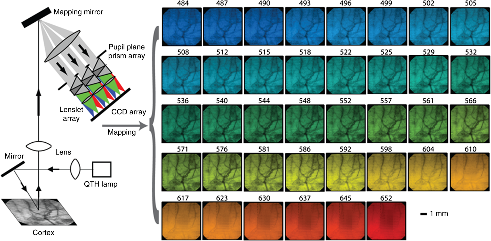

2.4.

Data Analysis

2.4.1.

Intrinsic signal

For each block of 64 trials, we averaged the imaged reflectance at each time point over the 64 trials. For each time point, the averaged data set consisted of a data cube consisting of 38 $350\times 350\text{pixel}$ images, with each image corresponding to one wavelength bin. We averaged the three exposures immediately preceding stimulation onset to calculate the baseline intensity. The intrinsic signal for each time point was then calculated for each pixel and wavelength separately as $\phi (t)=\log [R(t)/R_0]$, where $R(t)$ and $R_0$ are the measured light intensity at time $t$ and the baseline intensity, respectively. We related the intrinsic signal $\phi (t)$ to the changes in oxy- and deoxyhemoglobin in the cortex resulting from sensory stimulation using both the modified Beer–Lambert law and the Rytov approximation.

2.4.2.

Modified Beer–Lambert law

In order to generate 2-D images of the changes in hemoglobin concentrations, we used the modified Beer–Lambert law, which appears as

Eq. (1)

$$\phi (t)=-[{ϵ}_{{\mathrm{HbO}}_2}(\lambda )\delta {\mathrm{ctHbO}}_2(t)+{ϵ}_{\mathrm{Hb}}(\lambda )\delta \mathrm{ctHb}(t)]L(\lambda ).$$

Here, ${ϵ}_{{\mathrm{HbO}}_2}$ and ${ϵ}_{\mathrm{Hb}}$ are the extinction coefficients for oxy- and deoxyhemoglobin,⁵¹ $\delta {\mathrm{ctHbO}}_2(t)$ and $\delta \mathrm{ctHb}(t)$ are the changes in tissue concentration of those chromophores relative to their baseline values, and $L(\lambda )$ is the mean photon path length in the cortex as a function of wavelength. Monte Carlo simulations were used to determine the mean path lengths traveled by photons of differing wavelengths. In our Monte Carlo simulations, we began by using tissue oxy- and deoxyhemoglobin concentrations of ${\mathrm{ctHbO}}_2=60\mu \mathrm{M}$ and $\mathrm{ctHb}=40\mu \mathrm{M}$, respectively, tissue-scattering coefficient of ${\mu }_{\mathrm{s}}=10{\mathrm{mm}}^{-1}$, and tissue-scattering anisotropy of $g=0.9$, similar to values we have measured previously in this animal model using quantitative spatial frequency domain imaging.⁵²

2.4.3.

Rytov approximation

While the modified Beer–Lambert law has been used extensively to produce images of changes in hemoglobin concentration, Eq. (1) assumes that the changes occur uniformly throughout the brain. The Rytov approximation is a generalization of the modified Beer–Lambert law that allows one to solve for spatially varying changes in chromophore concentrations.⁵³ By taking advantage of the differing penetration depths of visible and near-infrared light in the cortex, we can implement the Rytov approximation to generate 3-D images of the changes in Hb and ${\mathrm{HbO}}_2$ concentrations.

The propagation of multiple-scattered incoherent light in tissue is governed by the radiative transport equation (RTE)

Eq. (2)

$$\widehat{\mathbf{s}}·\nabla I(\mathbf{r},\widehat{\mathbf{s}})+{\mu }_{\mathrm{t}}I(\mathbf{r},\widehat{\mathbf{s}})={\mu }_{\mathrm{s}}\int {\mathrm{d}}^{2}sA(\widehat{\mathbf{s}},{\widehat{\mathbf{s}}}^{\prime })I(\mathbf{r},\widehat{\mathbf{s}})+S(\mathbf{r},\widehat{\mathbf{s}}),$$

where $I(\mathbf{r},\widehat{\mathbf{s}})$ is the specific intensity, ${\mu }_{\mathrm{a}}$ and ${\mu }_{\mathrm{s}}$ are the absorption and scattering coefficients, respectively, ${\mu }_{\mathrm{t}}={\mu }_{\mathrm{a}}+{\mu }_{\mathrm{s}}$ is the extinction coefficient, $A(\widehat{\mathbf{s}},{\widehat{\mathbf{s}}}^{\prime })$ is the phase function, and $S(\mathbf{r},\widehat{\mathbf{s}})$ describes the source. The RTE allows us to relate the changes in light intensity detected at location ${\mathbf{\rho }}_{\mathrm{d}}$ in direction ${\mathbf{s}}_{\mathrm{d}}$ to changes in the concentrations of Hb and ${\mathrm{HbO}}_2$, by use of the Rytov approximation

Eq. (3)

$$\phi (\lambda ,{\mathbf{\rho }}_{\mathrm{d}},{\widehat{\mathbf{s}}}_{\mathrm{d}})=-\int {\mathrm{d}}^{3}r{\mathrm{d}}^{2}sI(\lambda ,z,\widehat{\mathbf{s}})G(\lambda ,\mathbf{r},\mathbf{s},{\mathbf{r}}_{\mathrm{d}},{\widehat{\mathbf{s}}}_{\mathrm{d}})\delta {\mu }_{\mathrm{a}}(\lambda ,\mathbf{r}),$$

where

Eq. (4)

$$\phi (\lambda ,{\mathbf{\rho }}_{\mathrm{d}},{\widehat{\mathbf{s}}}_{\mathrm{d}})=I(\lambda ,z=0,\widehat{\mathbf{s}})\log \left[\frac{R(\lambda ,{\mathbf{\rho }}_{\mathrm{d}},{\widehat{\mathbf{s}}}_{\mathrm{d}})}{R_0(\lambda ,{\mathbf{\rho }}_{\mathrm{d}},{\widehat{\mathbf{s}}}_{\mathrm{d}})}\right]$$

is the data function, $I(\lambda ,z,\widehat{\mathbf{s}})$ is the specific intensity of the planar illumination in the cortex, $G(\lambda ,\mathbf{r},\mathbf{s},{\mathbf{r}}_{\mathrm{d}},\mathbf{n})$ is the Green’s function for the RTE, and the change in absorption is decomposed into a sum of the contributions from changes in ctHb and ${\mathrm{ctHbO}}_2$

Eq. (5)

$$\delta {\mu }_{\mathrm{a}}(\lambda ,\mathbf{r})={ϵ}_{\mathrm{Hb}}(\lambda )\delta \mathrm{ctHb}(\mathbf{r})+{ϵ}_{{\mathrm{HbO}}_2}(\lambda )\delta {\mathrm{ctHbO}}_2(\mathbf{r}).$$

We solve Eq. (4) using a correction to the standard diffusion approximation that accounts for the fact that near boundaries, the specific intensity is not isotropic.^54,55 Using this correction, we can rewrite Eq. (4) as

Eq. (6)

$$\phi (\lambda ,{\mathbf{\rho }}_{\mathrm{d}})=\int {\mathrm{d}}^{3}r[I(\lambda ,z)G(\lambda ,\mathbf{r},{\mathbf{r}}_{\mathrm{d}})-\frac{\ell {*}^2}{3}\nabla I(\lambda ,z)·\nabla G(\lambda ,\mathbf{r},{\mathbf{r}}_{\mathrm{d}})]c\delta {\mu }_{\mathrm{a}}(\lambda ,\mathbf{r}).$$

Here, $I(\lambda ,z)$ is the photon density, $\ell *=1/({\mu }_{\mathrm{a}}+{\mu }_{\mathrm{s}}^{\prime })$ is the transport mean free path, $c$ is the speed of light, ${\mathbf{\rho }}_{\mathrm{d}}$ is a 2-D vector specifying the detector location, and the Green’s function $G(\lambda ,\mathbf{r},{\mathbf{r}}^{\prime })$ satisfies the diffusion equation

Eq. (7)

$$[D(\lambda ){\nabla }^2+c{\mu }_{\mathrm{a}}(\lambda )]G(\lambda ,\mathbf{r},{\mathbf{r}}^{\prime })=\delta (\mathbf{r}-{\mathbf{r}}^{\prime }),$$

with the diffusion coefficient $D=c\ell */3$. In Eq. (6), we have assumed that the source and detected light are orientated normal to the tissue surface.

Equation (7) is the most easily inverted in the Fourier domain where it is block diagonal. Taking a 2-D Fourier transform with respect to the detector position ${\mathbf{\rho }}_{\mathrm{d}}$ yields a 1-D integral for each value of the Fourier coefficient $\mathbf{q}$

Eq. (8)

$$\tilde{\phi }(\lambda ,\mathbf{q})=\int \mathrm{d}z\kappa (\lambda ,\mathbf{q},z)\delta {\tilde{\mu }}_{\mathrm{a}}(\lambda ,\mathbf{q},z).$$

The function $\kappa (\lambda ,\mathbf{q},z)$ can be calculated from Eq. (7) using known expressions for the Green’s functions of the diffusion equation. ⁵⁵ In the semi-infinite geometry, we have

Eq. (9)

$$\kappa (\lambda ,\mathbf{q},z)={\left(\frac{\ell }{D}\right)}^2[1-\frac{\ell {*}^2}{3}Q(\lambda ,q)Q(\lambda ,0)]\left(\frac{\exp \{[Q(\lambda ,q)+Q(\lambda ,0)]z\}}{[Q(\lambda ,q)\ell +1][Q(\lambda ,0)\ell +1]}\right),$$

where $\ell$ is the extrapolation length, defined as the distance from the boundary at which the energy density reaches zero,⁵⁶ and $Q(\lambda ,q)={(c{\mu }_{\mathrm{a}}/D+q^2)}^{1/2}$. The changes in ctHb and ${\mathrm{ctHbO}}_2$, relative to baseline, are then calculated according to

Eq. (10)

$$\delta \mathrm{ctHb}(\mathbf{\rho },z)=\int \frac{{\mathrm{d}}^{2}q}{{(2\pi )}^2}\exp (-i\mathbf{q}·\mathbf{\rho })\sum _{m,n}{ϵ}_{\mathrm{Hb}}({\lambda }_m)\kappa *({\lambda }_m,\mathbf{q},z)M_{m,n}^{-1}(\mathbf{q})\tilde{\phi }({\lambda }_n,\mathbf{q}),$$

Eq. (11)

$$\delta {\mathrm{ctHbO}}_2(\mathbf{\rho },z)=\int \frac{{\mathrm{d}}^{2}q}{{(2\pi )}^2}\exp (-i\mathbf{q}·\mathbf{\rho })\sum _{m,n}{ϵ}_{{\mathrm{HbO}}_2}({\lambda }_m)\kappa *({\lambda }_m,\mathbf{q},z)M_{m,n}^{-1}(\mathbf{q})\tilde{\phi }({\lambda }_n,\mathbf{q}).$$

We compute the matrix elements of $M(\mathbf{q})$ analytically according to

Eq. (12)

$$M_{m,n}(\mathbf{q})={\int }_0^{\infty }\mathrm{d}z[{ϵ}_{\mathrm{Hb}}({\lambda }_m){ϵ}_{\mathrm{Hb}}({\lambda }_n)+{ϵ}_{{\mathrm{HbO}}_2}({\lambda }_m){ϵ}_{{\mathrm{HbO}}_2}({\lambda }_n)]\kappa ({\lambda }_m,\mathbf{q},z)\kappa *({\lambda }_n,\mathbf{q},z),$$

and then find its inverse by solving its eigenvalue problem. The inversion is regularized by setting eigenvalues below a threshold to zero.

The framework of this Rytov-approximation-based algorithm has previously been shown to provide accurate estimates of depth of buried fluorescent inclusions in small animals.⁴⁶ In addition, we have recently performed a validation of the hyperspectral tomography algorithm on data generated using Monte Carlo simulations⁵⁷ with a 2-mm thick absorbing inclusion buried 0.5 mm beneath the surface. For this case (Fig. 2), the multispectral tomography algorithm was able to accurately reconstruct the center depth of the inclusion to within 23% and the inclusion thickness to within 18%. A more detailed discussion of tomography validation studies, employing both tissue-simulating phantoms and computational models of the forward problem, will be the subject of a future report (currently in preparation).

Fig. 2

Absorber concentration [averaged over a region of interest (ROI) and normalized to peak] as a function of depth, calculated for simulated data using the Rytov-approximation-based optical tomography algorithm described in Sec. 2.4.2. The data functions were generated by using Monte Carlo software⁵⁷ to simulate the two-dimensional surface reflectance at different wavelengths for a tissue model with a subsurface absorbing inclusion ($10\times$ the absorption of the surroundings) buried beneath 0.5 mm of tissue and having an extent of 2 mm in the $z$-direction (as denoted by the blue box overlaid on the figure). The reconstructed center depth of the inclusion was defined as the $z$-value at which the reconstructed concentration had its highest value. The reconstructed extent of the inclusion was defined as the full-width at half-maximum of the curve describing the concentration as a function of depth. For this case, the multispectral tomography algorithm reconstructed the center depth and thickness of the inclusion to within 23% and 18%, respectively.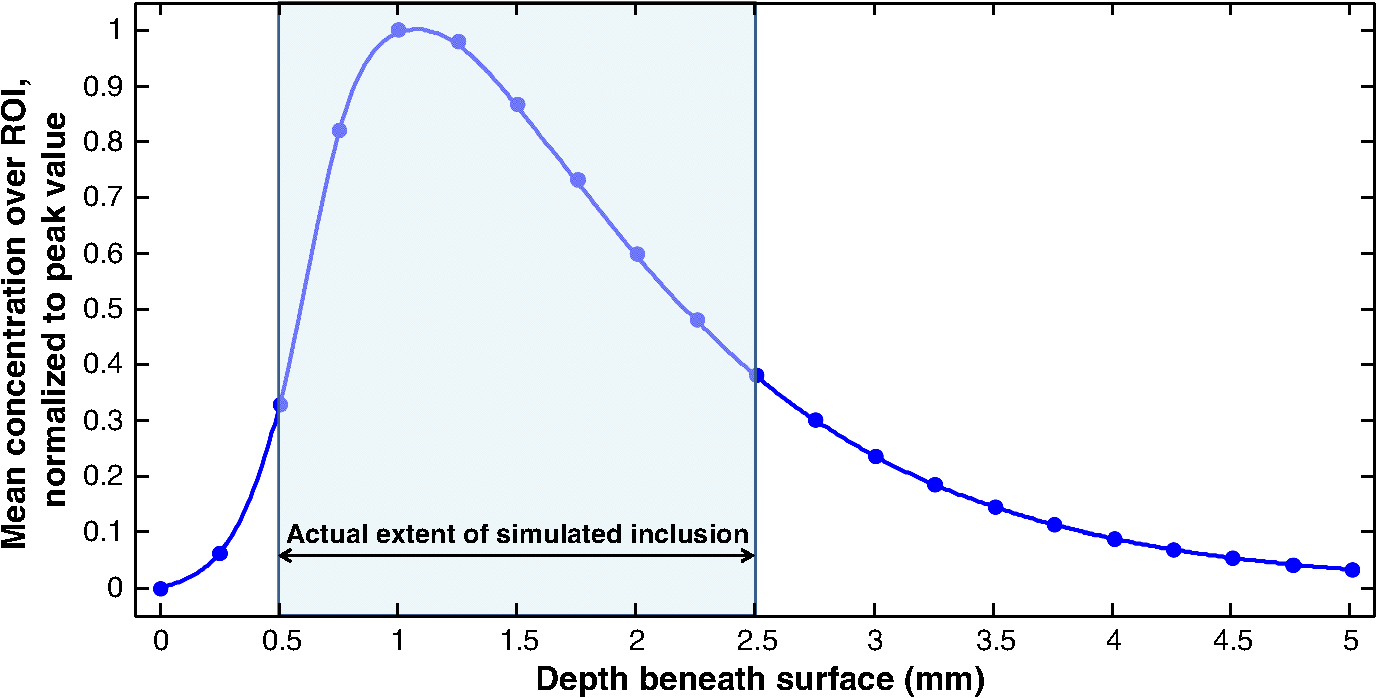

3.

Results and Discussion

Figure 3 demonstrates our ability to image the changes in light intensity due to functional activation with high spatial and temporal resolution simultaneously at many wavelengths through a thinned skull in a representative rat. Figure 3(a) shows images of changes in light remitted from the cortex at 529 nm (isosbestic point equally sensitive to oxy- and deoxyhemoglobin) and 630 nm (about $9\times$ more sensitive to deoxyhemoglobin than oxyhemoglobin).

Fig. 3

Imaging changes in light intensity. (a) Images of the cortex using 570 nm light are overlaid with color images representing the change in remitted light at 529 nm (isosbestic point sensitive to total hemoglobin concentration) and 630 nm (primarily sensitive to deoxyhemoglobin). Time points correspond to the initial decrease in signal at 630 nm, the decrease at 529 nm, and the overshoot at 630 nm. The purple/yellow color scale indicates an increase in remitted light, while the green/blue scale represents a decrease. (b) Time course of remitted light intensity for the ROI (see Sec. 2) at an isosbestic point (529 nm), deoxyhemoglobin peak (557 nm), oxyhemoglobin peak (576 nm), and at 630 nm. (c) Spectra of the intrinsic signal during the time points pictured in (a). (d) False color representation of intrinsic signal as a function of both time and wavelength. (e) Spectra of oxy- and deoxyhemoglobin. (b, c) Error bars represent the standard error over all pixels in the ROI. Regions of interest were determined by selecting a pixel in the 630 nm image where a maximum drop in measured light intensity occurred, and then averaging over a $500\mathrm{mm}\times 500\mathrm{mm}$ area surrounding that pixel.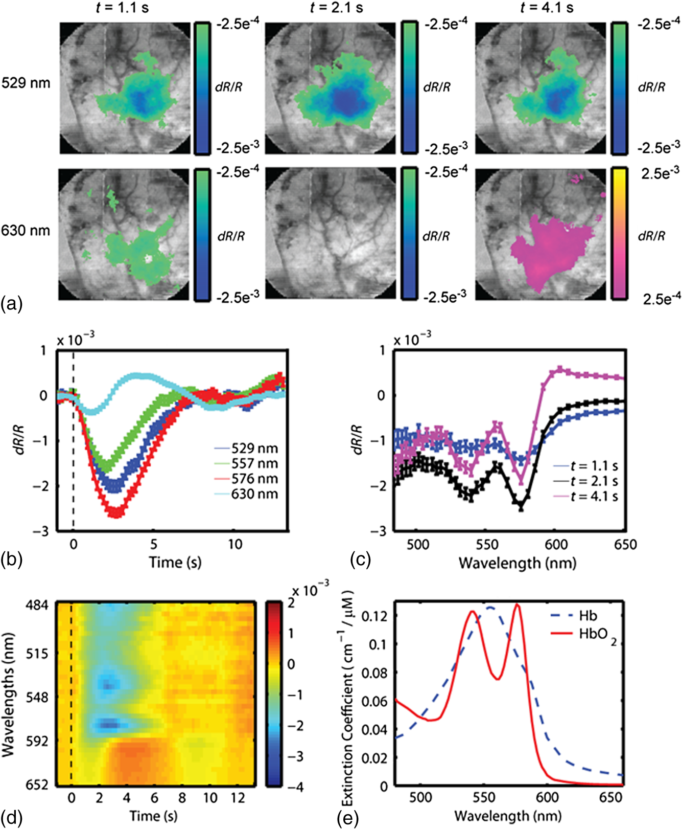

Color maps of the change in light intensity are superimposed over black and white images at 576 nm, which clearly show the underlying vasculature. As can be seen by looking at the time dependence of the signal over the area of peak activation shown in Fig. 3(b), the time points chosen in Fig. 1(a) correspond to the initial decrease in the 630 nm signal, the time at which the isosbestic wavelength (529 nm) has its largest signal, and the increase of signal at 630 nm. Complete spectral information for these three time points is shown in Fig. 3(c), and the intrinsic signal is represented in Fig. 3(d) in false color as a function of both wavelength and time. These results are in agreement with our previous ISOI imaging at a single wavelength.⁴⁸

Representative images of the changes in ctHb and ${\mathrm{ctHbO}}_2$ along with traces of the region of interest calculated using the modified Beer–Lambert law appear in Figs. 4(a) and 4(b). Changes in concentration (Table 1, averaged over all rats) were determined using the modified Beer–Lambert law, where optical path lengths were determined using Monte Carlo simulations of photon transport. The peak increase in ${\mathrm{ctHbO}}_2$ ($\delta {\mathrm{ctHbO}}_2=248\pm 80\mathrm{nM}$) was $\sim 3\times$ greater than the ctHb decrease ($\delta \mathrm{ctHb}=-84\pm 20\mathrm{nM}$). The peak changes in concentration did not occur at the same time; the peak change in total hemoglobin arose first ($t_{\mathrm{HbT}}=2.6\pm 0.4\mathrm{s}$), followed by the peak in ${\mathrm{ctHbO}}_2$ ($t_{{\mathrm{HbO}}_2}=3.1\pm 0.3\mathrm{s}$), and the maximum decrease in ctHb ($t_{\mathrm{Hb}}=4.3\pm 0.3\mathrm{s}$).

Fig. 4

Representative images of changes in concentration and with varied wavelengths. (a) Images of the change in tissue concentration of deoxy- and oxyhemoglobin for a representative rat at time points corresponding to the initial ctHb increase (1.1 s), the ${\mathrm{ctHbO}}_2$ increase (3.1 s), and the ctHb decrease (3.7 s), obtained using the modified Beer–Lambert law. Color maps of the hemoglobin changes are overlaid above an image of the cortex at 570 nm. The purple/yellow color scale indicates an increase in concentration, while the green/blue scale represents a decrease. (b, c) Time-resolved changes in ctHb and ${\mathrm{ctHbO}}_2$ for the ROI on the cortex, obtained using the modified Beer–Lambert law, for (b) all wavelengths and (c) only for the wavelengths 529 and 630 nm. Error bars represent the standard error for all pixels in the ROI.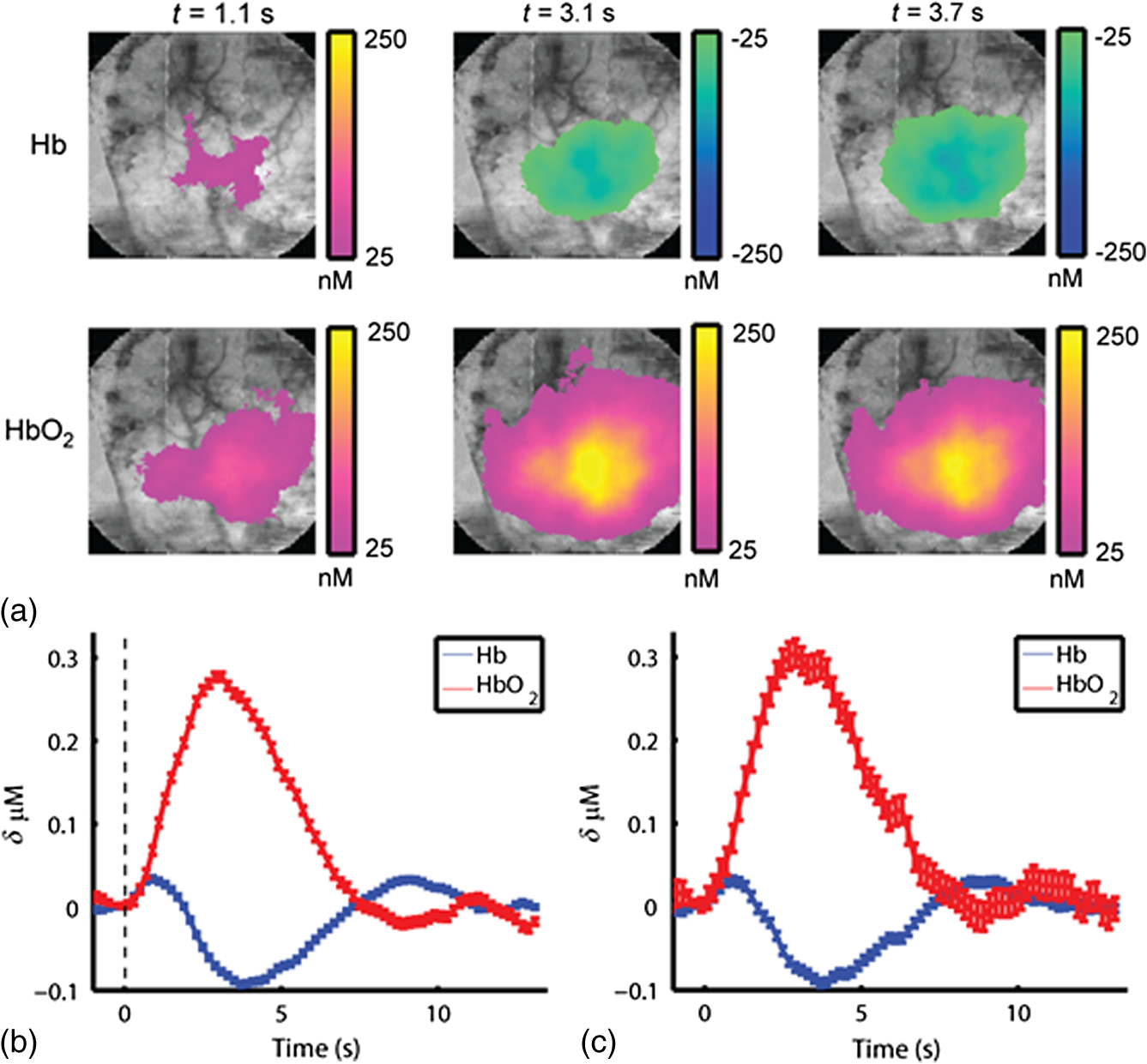

Table 1

Peak times and maximum changes in the concentrations of oxyhemoglobin (ctHbO2) and deoxyhemoglobin (ctHb) using the modified Beer–Lambert law and the Rytov approximation.

We varied the number of wavelengths used to fit for ctHb and ${\mathrm{ctHbO}}_2$ to determine the effect on the recovered changes in hemoglobin concentration. We found that using fewer wavelengths led to additional noise in the recovered hemoglobin values. For example, Figs. 4(b) and 4(c) shows the hemoglobin time courses for a single rat using all 38 wavelengths [Fig. 4(b)], and only using two wavelengths [Fig. 4(c)]: an isosbetic wavelength (529 nm) and a deoxyhemoglobin sensitive wavelength (630 nm). When reducing the number of wavelengths from 38 to 2, the standard error of hemoglobin concentration changes in the regions of interest increased from 6 to 20 nM for ${\mathrm{ctHbO}}_2$ and from 3.5 to 5.6 nM for ctHb. However, despite the increase in noise, removing wavelengths did not significantly alter the timing or peak magnitudes of the hemodynamic time courses.

We also conducted Monte Carlo simulations over a wide range of parameters to determine the effect of path length on the calculated values for changes in ctHb and ${\mathrm{ctHbO}}_2$. Figure 5 illustrates the variability in the magnitude of hemoglobin changes calculated when different baseline optical properties are assumed. The variability of the initial ctHb increase, the ${\mathrm{ctHbO}}_2$ increase, and the subsequent ctHb decrease are reported in Table 2. Increasing the baseline value of total hemoglobin or scattering leads to an increase in the magnitude of all parameters. This occurs because an increase in absorption or scattering decreases the mean photon path length. Since the data remain fixed, this leads to an increase in the calculated hemoglobin concentrations (see Sec. 2). All changes due to varying the wavelength dependence of scattering, described by $A{\lambda }^{-b}$ where the $A$ and $b$ parameters refer to scattering amplitude and power, respectively,^46,52 were less than 15% despite changing scattering power, $b$, over a large range ($b=0–2.5$).

Table 2

Magnitude of changes in hemoglobin concentrations for the differing optical properties used in the Monte Carlo simulations.

Fig. 5

Time courses for the concentrations of oxy- and deoxyhemoglobin, averaged over all rats, where the optical properties have been varied when determining the mean photon path length used in the modified Beer–Lambert law. The values of (a) total tissue hemoglobin concentration (HbT), (b) tissue hemoglobin oxygenation (${\mathrm{StO}}_2$), (c) scattering coefficient (${\mu }_{\mathrm{s}}$), and (d) scattering power ($b$ parameter, see text) were varied. Error bars indicate the standard error for all rats.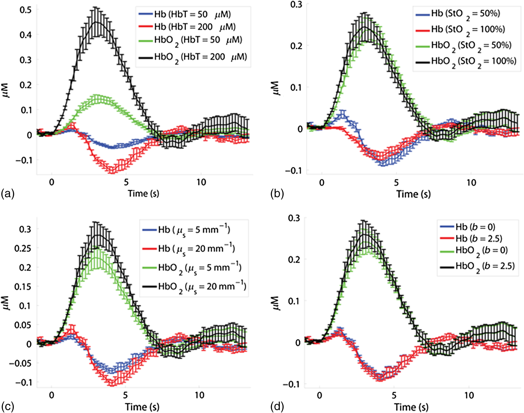

Future work will include a quantitative comparison between the tomography model used in this paper and a Monte Carlo-based tomography model that uses photon path length information stored in the simulations to provide accurate quantification of absorber depth and concentration. Future work will also include a detailed computational investigation into the influence of tissue background absorption and scattering properties on the depth sensitivity of the optical tomography algorithm. This future study will also include a systematic investigation into how the background optical properties and the set of wavelengths employed affects the ability of the algorithm to fully separate oxygenated hemoglobin absorption from deoxygenated hemoglobin absorption. This future work will include a quantitative comparison between the tomography model used in this paper and a Monte Carlo-based tomography model that uses photon pathlength information stored in the simulations to provide accurate quantification of absorber depth and concentration.

Figure 6 shows representative depth-resolved snapshots of the changes in oxy- and deoxyhemoglobin at 4 s poststimulus for one rat. These images were calculated according to the Rytov approximation method described in Sec. 2.4.2. Eleven wavelengths from 586 to 652 nm were employed in the reconstructions. Slices of the 3-D images of ctHb and ${\mathrm{ctHbO}}_2$ are shown at six depths from $100\mu \mathrm{m}$ to 1.1 mm beneath the surface of the cortex. Depth profiles of the changes in oxy- and deoxyhemoglobin, as a function of depth beneath the surface of the cortex, are shown in Fig. 7(a) for the same rat as in Fig. 6. Figure 7(b) shows time courses of these changes in oxy- and deoxyhemoglobin, at a depth of 0.3 mm beneath the surface of the cortex, averaged over four rats.

Fig. 6

Representative three-dimensional reconstructed images of changes in oxy- and deoxyhemoglobin for one rat in response to stimulus, obtained at time $t=4\mathrm{s}$ poststimulus using the Rytov approximation. Each panel represents a cross section at a given depth beneath the surface of the cortex. The concentration maps have been overlaid on 571-nm reflectance images of a $4.35\mathrm{mm}\times 4.35\mathrm{mm}$ region of the cortex.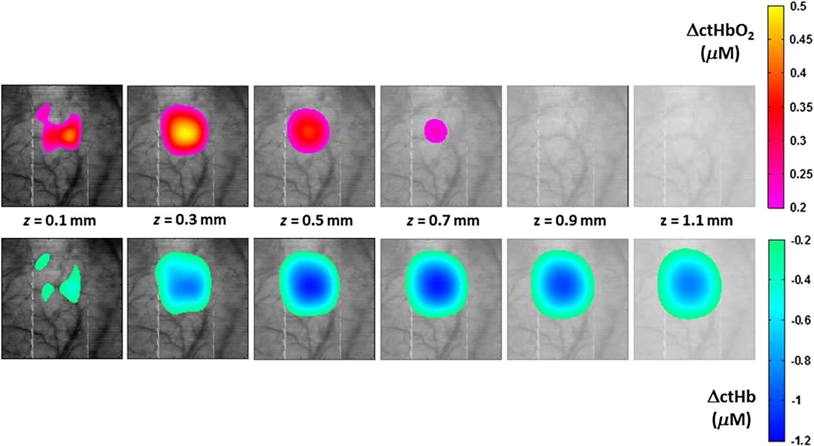

Fig. 7

Depth profiles of changes in oxy- and deoxyhemoglobin concentrations in response to stimulus (a) at time $t=4\mathrm{s}$ poststimulus, for the same rat as in Fig. 6, shown alongside a schematic of the rat cortical layers (based on Ref. 58), on the same scale as the depth profile plot. The changes in oxy- and deoxyhemoglobin were primarily confined to layers 2 to 4 of the cortex. (b) Time courses of changes in ${\mathrm{ctHbO}}_2$ and ctHb poststimulus, obtained at a depth of 0.3 mm beneath the surface of the cortex (the depth of peak change in oxyhemoglobin concentration), using the Rytov approximation, averaged over four rats (error bars represent the standard error).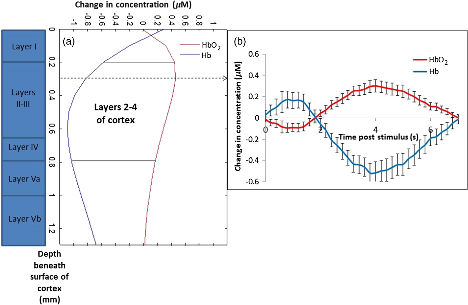

The time courses shown in Fig. 7(b) illustrate an initial decrease in the concentration of oxyhemoglobin and an initial increase in the concentration of deoxyhemoglobin over the first 2 s poststimulus, followed by an increase in the oxyhemoglobin concentration and a decrease in the deoxyhemoglobin concentration over the subsequent 5 s. Using the Rytov tomography algorithm, the maximum changes in ${\mathrm{ctHbO}}_2$ and ctHb were found to occur at depths of $0.29\pm 0.02$ and $0.66\pm 0.04\mathrm{mm}$ beneath the surface of the cortex, respectively. The peak times and magnitudes of concentration changes for the 3-D image reconstructions are summarized in Table 1. For the Rytov tomography algorithm, the point of peak concentration change (Table 1) was defined as the peak time point at the depth ($z=0.3\mathrm{mm}$ beneath the surface of the cortex) at which the peak change in oxyhemoglobin concentration occurred. The magnitudes of the peak changes in oxy- and deoxyhemoglobin concentration shown in Table 1 are larger for the Rytov tomography algorithm than the Beer–Lambert method; this finding is expected because the Rytov tomography algorithm localizes the changes in 3-D space.

The results shown in Figs. 6 and 7 are indicative of the depletion of oxygen by the cortex in response to the stimulus, followed by the reperfusion of oxygenated blood into the region. Figures 6 and 7 also suggest that the relative magnitudes of the changes in oxy- and deoxyhemoglobin may vary with depth. This effect could possibly be explained by differences in depth of diving arterioles and venuoles, with the extraction of oxygen occurring deeper in the cortex and the reperfusion of oxygenated blood occurring closer to the surface. However, this effect may also represent a limitation of the ability of the measurement technique and/or mathematical model to fully resolve the depths of two different absorbers (oxy- and deoxyhemoglobin), whose spectral features are close together in the interrogated wavelength range.

It is important to note that the peak magnitudes of concentration change were higher in the 3-D tomographic images (using the Rytov approximation) than for the modified Beer–Lambert law analysis. This is not surprising since the modified Beer–Lambert law results represent a depth-averaged hemodynamic change, while the tomographic results localize this information. When the reconstructed 3-D maps of concentration changes were averaged over depths from 0.1 to 1.3 mm beneath the surface of the cortex to create 2-D maps of changes in oxy- and deoxyhemoglobin, the magnitude of the change in oxyhemoglobin concentration decreased to $154\pm 29\mathrm{nM}$, but the change in deoxyhemoglobin concentration remained essentially the same as in the 3-D map ($555\pm 99\mathrm{nM}$). This result is related to the inability of the Rytov tomography algorithm to localize the changes in deoxyhemoglobin concentration as precisely as the changes in oxyhemoglobin concentration (Figs. 6 and 7). This discrepancy could be due in part to the fact that the absorption features of oxy- and deoxyhemoglobin were not completely decoupled from each other due to the size of the wavelength bands detected by the image mapping spectrometer. Future studies will quantitatively examine this issue by convolving the oxy- and deoxyhemoglobin absorption spectra with the bandwidth profile $\mathrm{\Delta }\lambda (\lambda )$ of the detector.

4.

Conclusion

We have employed a parallel hyperspectral imaging technique, IMS, to record intrinsic optical signals in the rat somatosensory cortex over 38 wavelength bands (from 484 to 652 nm) at 5 Hz following mechanical movement of a single whisker. This approach was combined with a hyperspectral optical tomography algorithm to quantify and localize time-dependent concentration changes in oxygenated and deoxygenated hemoglobin that are characteristic of the response to the evoked stimulus. Our image reconstruction algorithm uses the Rytov approximation and takes advantage of the fact that the measured spectral changes in reflectance have a strong depth-dependent distortion. Data were also analyzed using a modified Beer–Lambert law in which the photon pathlength was accounted for using Monte Carlo modeling.

The Rytov approach revealed that the maximum measured changes in ${\mathrm{ctHbO}}_2$ and ctHb were primarily confined to layers II–IV of the cortex. However, the depth distribution of the Rytov-calculated ctHb change had a broader tail than that of the ${\mathrm{ctHbO}}_2$ change. Rytov tomographic reconstructions revealed spatially localized increases and decreases in ${\mathrm{ctHbO}}_2$ and ctHb of $321\pm 53$ and $555\pm 96\mathrm{nM}$, respectively, at $4\pm 0.2\mathrm{s}$ poststimulus. The modified Beer–Lambert model revealed a $248\pm 80\mathrm{nM}$ increase in ${\mathrm{ctHbO}}_2$ at $3.1\pm 0.3\mathrm{s}$ poststimulus and an $84\pm 19\mathrm{nM}$ decrease in ctHb at $4.3\pm 0.3\mathrm{s}$ poststimulus.

Localized optical BOLD signals for both ${\mathrm{ctHbO}}_2$ and ctHb were greater using the Rytov approximation than those estimated using the modified Beer–Lambert approach. One contribution to these differences in signal magnitude likely comes from the inability of planar reflectance methods to account for partial volume effects. The additional discrepancy between the ctHb values calculated with the Rytov and Beer–Lambert approaches is likely an artifact of the inability of the algorithm to completely separate the signal contributions from oxy- and deoxyhemoglobin. This is due, in part, to the fact that we did not rigorously characterize the effect of the wavelength dependence of detector bandwidth $\mathrm{\Delta }\lambda (\lambda )$. Future studies will investigate potential improvements to the Rytov model as well as imposing further optical path length constraints through the use of structured light projection patterns.^45,46 Despite these limitations, this study provides, for the first time, a general framework for localizing and characterizing hemodynamic signals in the cortex with $\sim \mathrm{mm}$ resolution over a wide, scalable field of view. One application of great potential biomedical importance is to employ multispectral optical tomography in combination with spatial frequency domain and laser speckle contrast imaging methods in order to separate the hemodynamic effects of blood flow from metabolism in the brain. These studies are currently in progress in our laboratory, with emphasis on characterization of the brain’s response to traumatic perturbations such as cardiac arrest and stroke in preclinical animal models.