2.1.

System Description

A PMF-based OCT system (Fig. 1) was used for cross-sectional imaging of neural activity. The light source is a 25-mW broadband near-infrared superluminescent diode (SLD) with a full-width half-maximum (FWHM) bandwidth of 50 nm centered at 840 nm (Broadlighter S840, Superlum, Ireland), yielding an axial resolution of $\sim 5.5\mu \mathrm{m}$ in tissue. After passing through a polarizer in the fiber bench, linearly polarized light is coupled to one of the orthogonal channels of PMF and then split into reference (70%) and sample (30%) arms by a $2\times 2$ polarization-maintaining (PM) coupler (Canadian Instrumentation and Research Ltd., Canada).

Fig. 1

Optical setup. SLD–superluminscent diode, PC–polarization controller, C–collimator, P–polarizer, FB–fiber bench, PM–polarization maintaining, QWP–quarter-wave plate, WP1, WP2–wave plates for maintaining linear polarization, DM–dichroic mirror, L–lens, R–partial reflector, G–transmission grating, WP–Wollaston prism, LSC–line scan camera.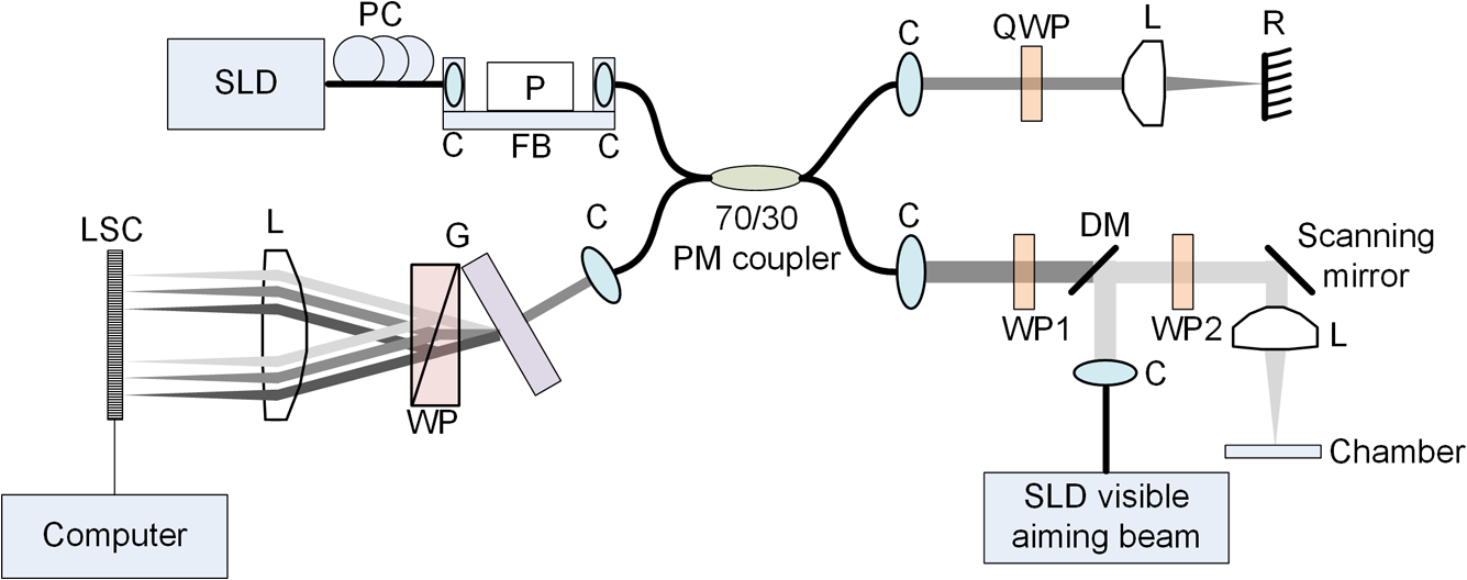

In the reference arm, collimated light passes through a quarter-wave plate oriented at 22.5 deg with respect to the PMF channel and an achromatic lens ($f=30\mathrm{mm}$), and returns from a reflector, which is the front surface of a glass wedge. As in conventional polarization-sensitive OCT,³² the returning light becomes linearly polarized at 45 deg; and therefore, equally couples back to the fast and slow axis of PMF. In the sample arm, light from 690 nm SLD and 840 nm system are combined by a dichroic mirror (T760 lpxr, cut-off wavelength: 760 nm, Chroma Technology Corp., Bellows Falls, Vermont). This configuration was already setup from another study and for this experiment visible light was only used for positioning the sample prior to data acquisition. A galvanometer-controlled mirror (Model 6215H, Cambridge Technologies, Cambridge, Massachusetts) directs the light onto the nerve, the axis of which was aligned 45 deg to the light polarization. Polarization effects of imperfect optical components in the sample arm are minimized by using wave plates before and after the dichroic mirror yielding about 22 dB isolation between the main and cross-polarized channels. The phase measurements from the squid nerve, which has low birefringence, do not require polarization sensitivity, as the phase information is obtained from the main channel. A 19-mm focal-length lens focuses the beam on the sample which resulted in $\sim 8.5\mu \mathrm{m}$ lateral resolution.

Light returning from the reference and sample arms mixes in the PM coupler. The interference occurs when the optical path difference between these arms is within the imaging depth. The PM fiber directs the interferometric signal in its slow and fast channels to a high-speed custom-built spectrometer. In the spectrometer, light collimated by an achromatic lens ($f=75\mathrm{mm}$) is dispersed to its spectral components by a $1200\text{lines}/\mathrm{mm}$ transmission grating (Wasatch Photonics, Logan, Utah). A Wollaston prism (Karl Lambrecht Corp., Chicago, Illinois) with a 6-deg splitting angle separates the two channels, which are then focused by an achromatic lens ($f=200\mathrm{mm}$) onto a CMOS line-scan camera (Sprint, spl4096-140 km Basler, Ahrensburg, Germany). Since the spectra of the main and cross channels are positioned side-by-side, a single acquisition of the camera is sufficient to capture the interference-related spectral oscillations on both channels (1024 pixels per channel with $2\times 2$ binning). The spectrometer was calibrated with a commercial spectrometer ($\mathrm{HR}2000+$, Ocean Optics, Dunedin, Florida) by using a diffraction grating coupling selected wavelengths of the light source to these spectrometers and fitting the readings to a curve.³³

The spectra carrying interference-related oscillations on both PMF channels were simultaneously acquired at the rate of 66.67 kHz ($15\mu \mathrm{s}/\mathrm{A}\text{-}\text{Line}$). The galvanometer-controlled mirror was scanning a triangular wave with a 0.5 ms period continuously during the acquisition for 16 ms. The optical power on the sample was 1 mW (power per unit area: $\sim 4.4\mu \mathrm{W}/\mu {\mathrm{m}}^2$). An isolated pulse stimulator (Model 2100, A-M Systems, Sequim, Washington) was used to deliver electrical current pulses of varying amplitudes to the squid nerve for a duration of $50\mu \mathrm{s}$. Electrical signals from the nerve were amplified and simultaneously recorded by an AC differential amplifier (Model 1800, A-M Systems, Sequim, Washington) and a data acquisition card (PCI 6110, National Instruments, Austin, Texas), respectively. The action potential traces were displayed on the oscilloscope to monitor the nerve functionality over time.

2.2.

Animal Preparation

Live squids (Loligo pealeii) were obtained and dissected at the Marine Biological Laboratory, Woods Hole, Massachusetts. The giant axon together with surrounding small fibers was extracted under a microscope. The solution was seawater. The staining was with an oxonol voltage-sensitive dye NK3630 (RH482, from Nippon Kankoh-Shikiso Kenkyusho Co., Ltd., Japan) $0.25\mathrm{mg}/\mathrm{mL}$ with 1% DMSO for 20 min in a dark environment. The nerve, stained or unstained, was placed in the nerve chamber and covered by a glass window in order to provide a reference surface for phase measurements.

2.3.

Electrical Stimulation and Functional Imaging

Detailed nerve chamber design and electrode recording settings can be found in Ref. 8. The linear light polarization impinged 45 deg (or 135 deg) to the long axis of the nerve, which resulted in maximum cross-polarized light intensity.³⁴ The nerves were cooled for recording to prolong the viability of the nerve and increase action potential duration. The amplitude of the stimulus current pulses was 4 mA. The imaging system simultaneously provided both structural and functional information due to the high sampling rate of the line-scan camera and the small scan area which was repeatedly scanned rapidly (0.5 ms period).

To choose a location for probing the functional activity, we monitored the larger cross-sectional scanning range of the squid nerve in the nerve chamber [Fig. 2(a)] The arrow indicates the axis of symmetry of the cross-sectional images as we apply one cycle of the triangular wave to the galvanometer. The black dashed lines of Fig. 2(a) show the approximate location of the smaller range functional scanning. A $20\text{-}\mu \mathrm{m}$ outer sheath was observed between the giant axon and the small nerve fibers of the stained squid nerve. The dark sloping line near the top is the glass–solution interface. The chamber was tilted to avoid saturation of specular reflection from glass surface. Once the area was selected, the smaller scanning range of the functional site [Fig. 2(b)] was recorded.

Fig. 2

OCT image (reflectivity contrast) of a squid nerve containing the small fibers and the giant axon (*) within a larger scanning range, (a) scale bars: $100\mu \mathrm{m}$. (b) The arrow indicates the axis of symmetry of the cross-sectional image and the black-dashed lines indicate the approximate location of small scan, scale bars: horizontal, $10\mu \mathrm{m}$; vertical, $100\mu \mathrm{m}$.

2.4.

Data Processing and Analysis

The spectra acquired by the line-scan camera for the orthogonal polarization channels were resampled to $k$-space and dispersion imbalance between the reference and sample arms was compensated in software. An inverse Fourier transform was then applied to the $k$-space spectra to obtain the complex-valued depth profiles, which are in the form of $A_{\mathrm{m}}(z)\exp [i{\phi }_m(z)]$, where $A$ is the amplitude and $\phi$ is the phase at a particular depth $z$, and the subscript $m$ refers to the channel number (1 or 2). The reflectivity information $R$ is proportional to the square of the amplitudes, as follows:

OCT images [Figs. 2 and 3] show the microstructure with the reflectivity contrast, typically in logarithmic scale. The images are formed by stacking several depth profiles acquired during lateral scanning of light over the sample. The phase of the complex depth profile allows quantification of optical path length variations at particular depths ($\mathrm{\Delta }p$ response). The phase values are affected by environmental perturbations changing the path difference between the reference and sample arms. Therefore, we removed the common-mode phase noise by subtracting the phase of a reference surface (glass–solution interface above the nerve) from the phase of the nerve locations. To calculate $\mathrm{\Delta }p(z)$, we used the phase of the main channel, ${\phi }_1$, as

Fig. 3

(a) Larger scope (scale bars: $100\mu \mathrm{m}$) and (b) smaller scope (scale bars: horizontal, $10\mu \mathrm{m}$; vertical, $100\mu \mathrm{m}$) of reflectivity showing the small fibers of a stained squid nerve. The smaller scope was repeatedly scanned for functional recording. The arrow indicates the turning point and the black-dashed lines show the approximate location of the smaller range functional scanning in (b).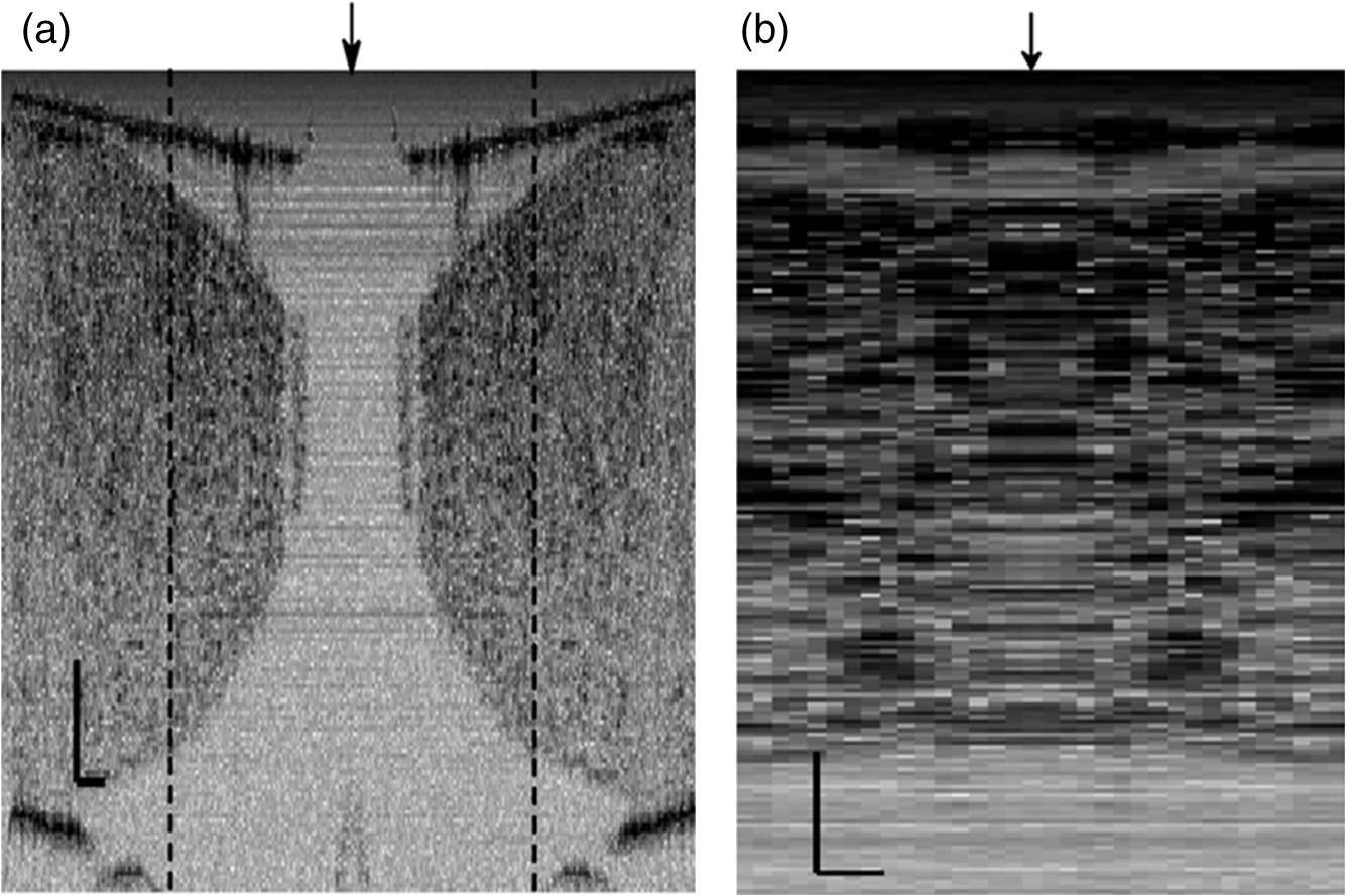

A functional back-and-forth scan consisted of 32 consecutive optical cross sections (32 triangular waves) during the recording. The scan range was adjusted by the amplitude of the triangular wave applied to the galvanometer controller. Optical contrasts of the cross section were acquired before, during, and after the action potential propagation. The signals for 10 and 90 responses were averaged to improve the SNR for analysis. A mask was created from the reflectivity image with a 25-dB threshold and applied to the phase image to exclude the low-SNR regions since low-reflection regions will result in unreliable phase values. To better illustrate the structural changes inside the squid nerve, the mean-subtracted absolute values of the $\mathrm{\Delta }p$ responses were taken due to the fact that the $\mathrm{\Delta }p$ responses can exhibit positive or negative deflections.

3.1.

Structural and Functional Imaging

The PMF-based OCT simultaneously provides the main channel backscattered light intensity, cross-polarized channel light intensity, the structural image [$R$, Eq. (1)], and the phase signals [$\mathrm{\Delta }p$, Eq. (2)] which may vary due to neural activity. Figures 3(a) and 3(b) depict the larger scope of reflectivity and the smaller scope of reflectivity with a dynamic range of 45 dB. The darkness of the structural image indicates the reflectivity from the squid nerve. This is a different location and a narrower region than Fig. 2. It is a region with only small nerve fibers of the stained nerve, whereas Fig. 2 shows the stained squid giant axon and small nerve fibers. The pixelated image in Fig. 3(b) contains fewer number of depth profiles (34 A-lines) due to the fast scanning speed, which is required for functional investigation. The reflectivity contrast shows the tissue light scattering properties of the squid small fibers within the smaller region of interest. Within the same measurement, the single-pixel reflectivity and phase, and their time-varying characteristics can be obtained.

3.2.

$\mathrm{\Delta }p$ Response

Figure 4 demonstrates the $|\mathrm{\Delta }p|$ response in cross-sectional slices before ($\sim 3\mathrm{ms}$), during ($\sim 8\mathrm{ms}$), and after ($\sim 12\mathrm{ms}$) the arrival of action potential to the measurement site. The electrical action potential recording is provided as well. A total of 90 trials ($N=90$) from a stained squid nerve were averaged to increase the SNR, although averaging 10 trials ($N=10$) was shown to be sufficient to visualize the activity (Fig. 5). The image size in Fig. 4 is about $90\mu \mathrm{m}\times 305\mu \mathrm{m}$. Considering two mirrored images, the actual scan range was $45\mu \mathrm{m}$ in the lateral direction. Since the galvanometer-controlled mirror was scanning a triangular wave signal for each cross section, the images show the mirror image at the turning point. The black arrow indicates the turning point found by postimage correlation. The cross-correlation of the ramp-up and ramp-down images within the acquisition time indicates that the lateral scanning was not drifting or shifting during the recording time. The conduction velocity of squid small fiber bundles is slower than the squid giant axon. The electrical current stimulation pulse was applied at $\sim 4\mathrm{ms}$ after the start of the recording, resulting in a stimulus artifact due to the residual current propagating from the stimulus electrodes to the recording electrodes. Unlike electrical recordings, optical recordings were free of stimulus artifacts. When the action potential reached the optical recording window at $\sim 8\mathrm{ms}$, the $|\mathrm{\Delta }p|$ response from multiple sites correspondingly occurred. The recovery after the action potential is shown at $\sim 12\mathrm{ms}$. The $|\mathrm{\Delta }p|$ response has not completely returned to baseline at $\sim 12\mathrm{ms}$, which is consistent with previous recordings with squid giant axons.⁸ We interpret the $\mathrm{\Delta }p$ signal shown in Fig. 4(b) as indicating regions of the fiber bundle that was active. Video 1 shows the $|\mathrm{\Delta }p|$ response for 16 ms.

Fig. 4

$|\mathrm{\Delta }p|$ response of a stained squid nerve at about (a) 3, (b) 8 and (c) 12 ms, and the corresponding action potential recording (scale bars: 0.2 mV). Stimulus is presented at about 4 ms. The arrows indicate the turning point of the galvanometer. Size of the region: $45\mu \mathrm{m}$ (from 0 to arrow) $\times 305\mu \mathrm{m}$. Ninety trials were averaged. Scale bars: horizontal, $10\mu \math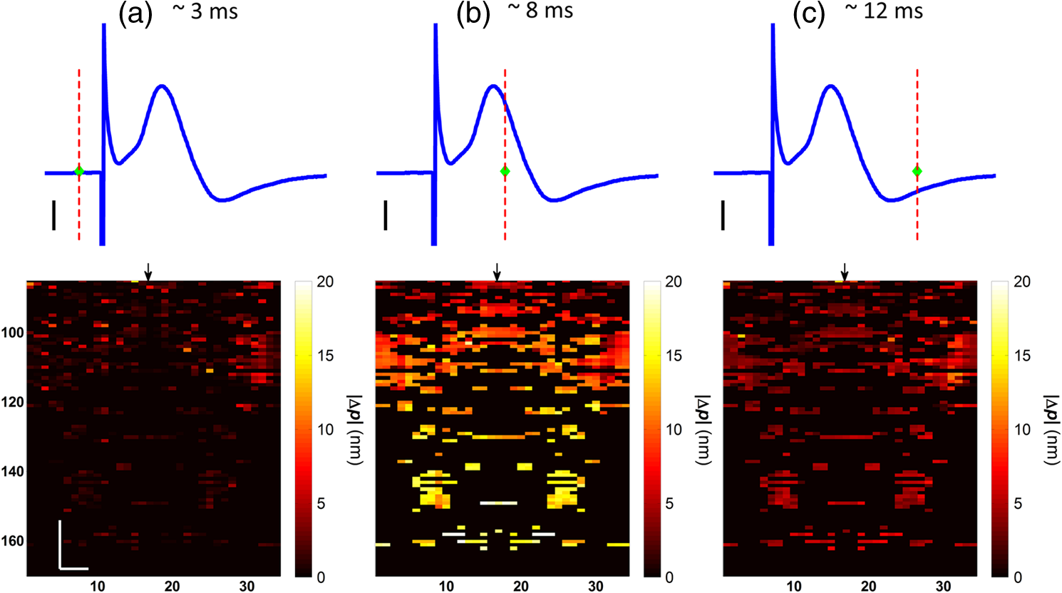rm{m}$; vertical, $50\mu \mathrm{m}$.

Fig. 5

Details of the $\mathrm{\Delta }p$ response. The data were also presented in Fig. 4. (a) Action potential, (b) $|\mathrm{\Delta }p|$ response at $\sim 8\mathrm{ms}$ is given by averaging 90 trials ($N=90$) and (c) 10 trials ($N=10$). In (b) and (c), arrow indicates the turning point of the galvanometer, and pixel numbers are given on the $x$-axis and $y$-axis. Scale bars: horizontal, $10\mu \mathrm{m}$; vertical, $100\mu \mathrm{m}$. Signal traces in time (d, e) are given for selected pixels (lateral index, depth index), which are marked by the blue circles in (b), with averaging 90 and 10 trials. Action potential traces in blue are for guidance. The cross sections for other time points are provided in Video 1 (Video 1, MOV, 3 MB) [DOI: http://dx.doi.org/10.1117/1.NPh.2.3.035001.1].

Figure 5 illustrates the action potential trace and the details of $\mathrm{\Delta }p$ response from the same scan. The red dashed line in Fig. 5(a) indicates the timing of the cross-sectional images. Figures 5(b) and 5(c) represent the $|\mathrm{\Delta }p|$ response at $\sim 8\mathrm{ms}$ by averaging 90 trials ($N=90$) and 10 trials ($N=10$), respectively. The image dimensions are about $90\mu \mathrm{m}\times 771\mu \mathrm{m}$. With the 10-trial average, the responses can be detected from the stained squid nerve. The cross sections for other time points are provided in Video 1. Since the absolute values of $\mathrm{\Delta }p$ signals were used, the functional cross-sectional images do not carry the sign information of the $\mathrm{\Delta }p$ responses. Figures 5(d) and 5(e) show the time course of the $\mathrm{\Delta }p$ response for selected pixels with $N=90$ and $N=10$, respectively. The actual locations of the pixels are given by pixel numbers in the coordinate system defined as (lateral index, depth index). The pixels are located at the center of the blue circles shown in Fig. 5(b). The images and the $\mathrm{\Delta }p$ traces are presented without spatial averaging. The action potential traces are given in blue for the time registration with the optical signals. Pixel (20,123) has the high standard deviation of the $\mathrm{\Delta }p$ signal during the 16 ms acquisition time. Pixels like these are masked out (dark pixels) in Figs. 5(b) and 5(c) due to the low reflectivity. Averaging multiple trials reduces the noise as shown in Figs. 5(d) and 5(e). The noise on the $\mathrm{\Delta }p$ measurement was analyzed for the prestimulus interval at multiple locations within five cross sections. Averaging 90 trials resulted in an $\sim 2.64$-fold improvement over averaging 10 trials, which agreed with the theoretical 3-fold improvement. Each pixel has a separate SNR value depending on the strength of the $|\mathrm{\Delta }p|$ response and the noise at that location. For pixels exhibiting $|\mathrm{\Delta }p|$ responses of 10 nm or more (range: 10–30 nm), the SNR was calculated by the ratio of the magnitude of the response (signal) and the standard deviation in the prestimulus interval (noise), which resulted in an average SNR of 6.7 for those pixels in Fig. 5 with averaging 10 trials.

Using another location of the same stained nerve, the $|\mathrm{\Delta }p|$ images at two different times and the $\mathrm{\Delta }p$ traces during the recording time for four pixels are demonstrated in Fig. 6. The results are averaged over 90 trials. Figure 6(a) shows the action potential trace with the red dashed lines at $\sim 7$ and $\sim 8.5\mathrm{ms}$ indicating the approximate timing of the $|\mathrm{\Delta }p|$ response presented in Figs. 6(b) and 6(c), respectively. The $|\mathrm{\Delta }p|$ images show different patterns as the activity arrives at the measurement sites within the cross section at different times. This is evident with the time traces of selected pixels in Fig. 6(d). Each $\mathrm{\Delta }p$ trace is obtained from a single pixel without spatial averaging. The pixels indicated by lateral index and depth index are located at the center of the blue circles marked in Fig. 6(b). Video 2 shows the response at other time points. Monophasic and biphasic signals were observed with increase and decrease phases in $\mathrm{\Delta }p$ response. Also, the maximum $\mathrm{\Delta }p$ responses occurred at different timing, e.g., $\sim 7–9\mathrm{ms}$. Interestingly, pixel (9,62) mainly shows the upward phase response, whereas pixels (17,64) and (21,121) show predominately downward phase responses. Typically, across all the recording sites, we observed that the $\mathrm{\Delta }p$ responses gradually change from upward to downward direction from the top to the deeper nerve areas. Also, pixels (11,64) and (17,64) have the same depth pixel index but different lateral pixel index corresponding to a separation of $\sim 16\mu \mathrm{m}$. The $\mathrm{\Delta }p$ responses of these pixels suggest different structural changes during the neural activity are happening within a very small range.

Fig. 6

(a) Action potential recording, (b) $|\mathrm{\Delta }p|$ images at $\sim 7\mathrm{ms}$, (c) $\sim 8.5\mathrm{ms}$ and (d) $\mathrm{\Delta }p$ traces of selected pixels recorded from a stained squid nerve. Ninety responses were averaged. Arrow indicates the turning point of the galvanometer. Scale bars in (b) and (c): horizontal, $10\mu \mathrm{m}$; vertical, $100\mu \mathrm{m}$. The blue circles in (b) are the actual locations plotted in (d). Pixel coordinates are given as (lateral index, depth index). The blue trace is the action potential recording for registering time. The $|\mathrm{\Delta }p|$ response at other time points is in Video 2 (Video 2, MOV, 2 MB) [DOI: http://dx.doi.org/10.1117/1.NPh.2.3.035001.2].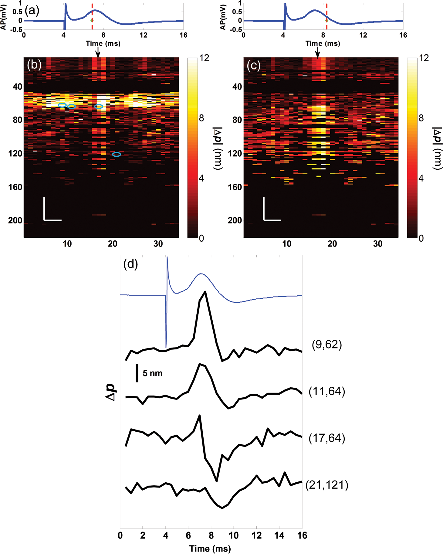

Without staining, we also observed the $\mathrm{\Delta }p$ responses from squid nerves. Figure 7 shows the $\mathrm{\Delta }p$ responses from an unstained nerve. The $|\mathrm{\Delta }p|$ image in Fig. 7(b) represents the response at $\sim 10.5\mathrm{ms}$. Video 3 shows the responses at other time points. The blue circles on the image are the actual locations plotted in Fig. 7(c). In this set of recordings, the scanning range ($90\mu \mathrm{m}$) was doubled compared to the stained case. This might result in a higher noise level due to wider range of scanning at the same scanning rate.

Fig. 7

(a) Action potential recording, (b) $|\mathrm{\Delta }p|$ image at $\sim 10.5\mathrm{ms}$ and (c) $\mathrm{\Delta }p$ traces of selected pixels from an unstained nerve with an averaging of 90 trials. Arrow in (b) indicates the turning point of the galvanometer mirror, scale bars: horizontal, $10\mu \mathrm{m}$; vertical, $100\mu \mathrm{m}$. Pixel coordinates in (c) are in the form of (lateral index, depth index), and the locations are marked by blue circles in (b). The blue trace is the action potential recording for the registering time. The $|\mathrm{\Delta }p|$ responses at other time points are in Video 3 (Video 3, MOV, 3 MB) [DOI: http://dx.doi.org/10.1117/1.NPh.2.3.035001.3].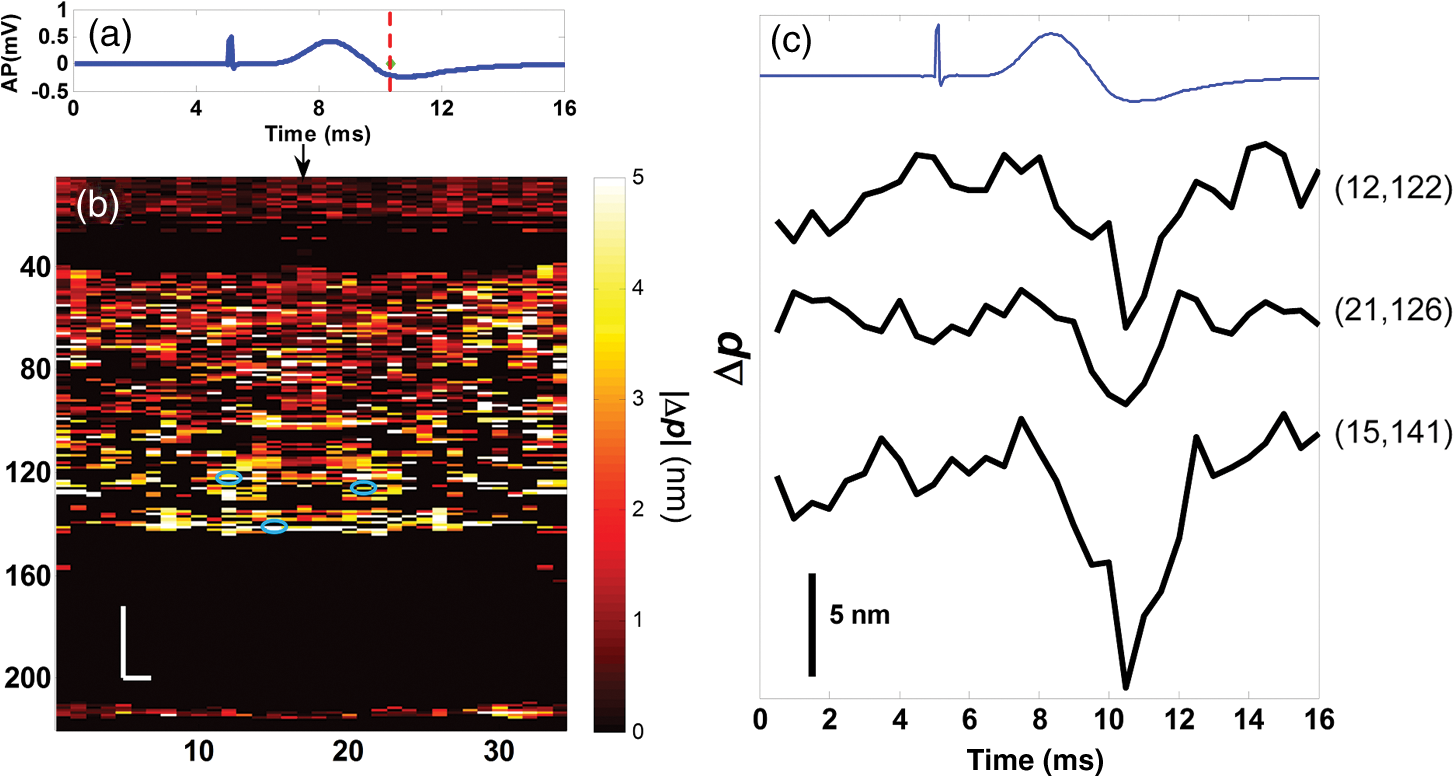

We chose five cross sections exhibiting $\mathrm{\Delta }p$ signals from a stained nerve and an unstained nerve to quantify and compare the transient response. Low SNR regions ($<25\mathrm{dB}$) were excluded from the analysis. During the action potential propagation, the mean and standard deviation of the single-pixel maximum $|\mathrm{\Delta }p|$ values for a stained and an unstained nerve were $5.54\pm 3.39\mathrm{nm}$ ($N=6834\text{pixels}$) and $4.01\pm 2.65\mathrm{nm}$ ($N=7638\text{pixels}$), respectively. On average, the $|\mathrm{\Delta }p|$ responses were larger from the stained nerve and their distribution was broader and more skewed toward larger values. Two of the cross sections, one presented here, for the stained nerve demonstrated larger $\mathrm{\Delta }p$ signals, but the other three cross sections were similar to the unstained values. Therefore, a potential effect of the dye on the $\mathrm{\Delta }p$ signals requires further investigation and the number of squids used in similar study should be increased.

3.3.

Assessments on Intensity and Phase Measurements

The PMF-based OCT system offers phase and intensity-based contrasts. For instance, the backscattering intensity on the main and cross-polarized channels forms reflectivity [$R$ from Eq. (1)]. These channels can also be used to analyze retardance/birefringence. In this study, we could not reliably obtain a detectable functional change on the intensity-based contrasts during neural activity. We analyzed the intensity signal on the main channel, $A_1(z)$, by randomly selecting 10 A-lines from a nerve cross section. The low SNR regions ($\text{reflectivity}<30\mathrm{dB}$) were excluded. The amplitude fluctuation due to perturbations such as vibrations and noise was calculated by the standard deviation divided by the mean of the peak values of the coherence functions. For a single trial, the amplitude fluctuation was 16.9% for the unstained nerves and 15.6% for the stained nerves. The numbers for M-mode imaging, 8.9% and 8.0%, showed better stability of the intensity measurements. Averaging 90 trials reduced the amplitude fluctuations due to perturbations for both unstained and stained nerves (2.5% and 3.1% for lateral scanning, and 1.8% and 2.2% for M-mode imaging, respectively).

Vibrations that change the optical path length difference between the reference and sample arms shift an entire depth profile up and down by a small amount with time. As a result, between the images there appears to have been bulk motion along the axis of the light beam due to mechanical noise. A stationary surface (glass–solution interface), with its phase multiplied by $\lambda /(4\pi )$, can be used to quantify the axial bulk motion. For a single trial, the standard deviation of this noise within 16 ms measurement time can exceed 10 nm (more with longer recordings). The $\mathrm{\Delta }p$ response did not suffer from this noise because of the differential operation. However, the intensity signal of a particular pixel could require software stabilization of the depth profile. After obtaining the axial bulk motion, we eliminated it from the images by reprocessing the spectral ($k$-space) data using the translation property of Fourier transform. However, fluctuations of the intensity signal due to other noise sources were much larger and action potential propagation signals could not be identified. In addition, the action potential-induced phase signals indicate local transient structural changes in the nerve, which can also influence the intensity signal. For instance, a 20 nm shift of a $5.5\mu \mathrm{m}$ wide Gaussian-shaped coherence function could induce a 0.004% fractional amplitude change at the peak, and $\sim 1\%$ change at the FWHM. These numbers are much smaller than the aforementioned amplitude fluctuation (noise); nevertheless, the effect of the $\mathrm{\Delta }p$ response can be decoupled from the intensity change when such a signal is detected.

To assess the sensitivity of the $\mathrm{\Delta }p$ measurement, we imaged a coverslip sample by both M-mode and cross-sectional scanning with the same experimental settings, and $\mathrm{\Delta }p$ was calculated from the phases of the top and bottom surfaces from the coverslip. The phase sensitivity is calculated as the standard deviation of this $\mathrm{\Delta }p$. Analyzing the $\mathrm{\Delta }p$ signals for each A-line over 16 ms recording time resulted in an average standard deviation of 425 pm within a cross section. The optical path length variation for both top and bottom surfaces of the coverslip (bulk motion) was much larger than the differential signal ($\mathrm{\Delta }p$) resulting in a common-mode rejection ratio of about 13 dB. The standard deviation for M-mode imaging was 341 pm. An unpaired student’s $t$ test showed that the standard deviations for M-mode and scanning configurations were not statistically significant ($p=0.21$). Due to surface nonuniformity in biological tissues, the sensitivity values for a nerve sample could degrade compared to a simpler structure. A potential advantage of scanning might be the reduction of light exposure onto the same nerve location, which might avoid photobleaching in some studies. Scanning also supports application of image processing techniques such as clustering and spatial averaging.