Network analysis of mesoscale optical recordings to assess regional, functional connectivity

Diana H. Lim; Jeffrey M. LeDue; Timothy H. Murphy

doi:10.1117/1.NPh.2.4.041405

22 June 2015 Network analysis of mesoscale optical recordings to assess regional, functional connectivity

Diana H. Lim, Jeffrey M. LeDue, Timothy H. Murphy

Author Affiliations +

Neurophotonics, Vol. 2, Issue 4, 041405 (June 2015). https://doi.org/10.1117/1.NPh.2.4.041405

Abstract

With modern optical imaging methods, it is possible to map structural and functional connectivity. Optical imaging studies that aim to describe large-scale neural connectivity often need to handle large and complex datasets. In order to interpret these datasets, new methods for analyzing structural and functional connectivity are being developed. Recently, network analysis, based on graph theory, has been used to describe and quantify brain connectivity in both experimental and clinical studies. We outline how to apply regional, functional network analysis to mesoscale optical imaging using voltage-sensitive-dye imaging and channelrhodopsin-2 stimulation in a mouse model. We include links to sample datasets and an analysis script. The analyses we employ can be applied to other types of fluorescence wide-field imaging, including genetically encoded calcium indicators, to assess network properties. We discuss the benefits and limitations of using network analysis for interpreting optical imaging data and define network properties that may be used to compare across preparations or other manipulations such as animal models of disease.

1. Introduction

A major goal in neuroscience is to map and understand the connectivity of the brain. Recently, there has been great interest in quantifying aspects of the connectome, which refers to a complete description of the structural or functional connections between elements of the nervous system.¹^,² There have been a number of efforts to reconstruct the structural connectivity of the entire brain through detailed anatomical tracing studies in the mouse³^–⁶ and rat⁷ brain. Such intense research effort is indicative of the great potential of the connectome to reshape our framework for understanding the brain in health and disease.⁸

Modern optical imaging techniques are generating large datasets from which anatomical or functional connectivity maps have been derived. Recently, network analysis (based on graph theory) has been used to describe these datasets as a type of network and to quantify their properties.¹^,⁹^–¹¹ Such analyses open exciting possibilities for experiments using network approaches to investigate the organizing principles of the brain,¹^,¹⁰ and have proven useful for quantifying how brain injury affects network structure and function.⁹^,¹²^,¹³ This tutorial will describe how we have applied network analysis and graph theory to optical imaging data [voltage-sensitive dye (VSD) imaging]. We provide sample data and analysis codes to illustrate the image processing and creation of brain network diagrams on our website, and refer to these throughout this tutorial.¹⁴

2. Why Use Network Analysis?

Perhaps the greatest advantage to use network analysis in neuroimaging research is that network analysis can take large, complex datasets and interpret it in a quantifiable way that lends itself to graphical presentation. Furthermore, network analysis can be applied to many different scales of connectivity studies ranging from the microscopic level (the level of neurons and synapses), to the mesoscopic level (the level of neuronal groups or populations), to the macroscopic scale (the global level of the entire brain and the inter-regional pathways between large cortical areas).⁸ At each of these levels, neural networks may be defined and described by quantifying important network properties (see Appendix for a brief overview or Ref. 15 for a full review of network properties). Network analysis can thus be applied to many different types of neuroimaging approaches, ranging from regional optical imaging¹²^,¹⁶^,¹⁷ to functional neuroimaging in a clinical setting using functional magnetic resonance imaging (fMRI).¹⁸ A connectomics approach to neuroimaging analysis allows for comparisons between structural and functional connectivity, as well as comparisons between subjects or groups. Network analysis has been shown to be useful in quantifying network changes that occur after brain injury, such as stroke,¹²^,¹⁸^,¹⁹ and may be useful in informing treatment and rehabilitation strategies or projecting recovery after brain injury. Network analysis may also prove to be useful in identifying changes that occur during aging, or in neurological diseases that do not have a well-defined etiology, such as schizophrenia²⁰ or autism spectrum disorder.²¹

3. Basic Concepts in Network Analysis

Networks are structures that consist of nodes (or vertices), and edges (or links) that connect nodes to one another. The number of links connected to a node is the node degree and broadly reflects the importance of the node within the network. Edges may be directed or undirected: directed edges may be anatomical or effective functional connections, and indicate that activity in one node modulates activity in the other node;²² undirected edges indicate an anatomical or functional connection between two nodes, but do not specify directionality for the edge, and there is no effective causality between the nodes¹⁵ [Fig. 1(a)]. In an undirected network the edges represent reciprocal connections, so the in-degree (the number of afferent connections for a given node) and out-degree (the number of efferent connections for a given node) is equal. In a directed network, edges are not necessarily reciprocal and the in-degree differs from the out-degree for each node (the number of connections to a given node does not necessarily equal the number of connections from that node) [Fig. 1(b)].

Fig. 1

Construction of network diagrams from connectivity matrices: (a) example of a simple unweighted (binary), undirected connectivity matrix and network. Note that the connectivity matrix is symmetrical across the diagonal because all edges are reciprocal ( $A \to B$ and $B \to A$ are equivalent); (b) example of a weighted, directed connectivity matrix and network. The thickness of the edges corresponds to the weight of the edge. Note that the edges in the network diagram display a direction (arrowheads), and connections between nodes are not always reciprocal (for example, while there is a strong efferent connection from D to A, there is no afferent connection from A to D).

Similarly, networks may be weighted or unweighted. Unweighted networks, also known as binary networks, simply indicate the presence or absence of an edge between two nodes [Fig. 1(a)]. On the other hand, weighted networks allow edges to be associated with a weight. The weight for each edge is typically proportional to the strength of the connection between the nodes [Fig. 1(b)].

Certain types of neuroimaging data lend themselves to particular network representations. For example, diffusion tensor imaging tractography and fMRI lend themselves to weighted, undirected networks as these data do not explicitly capture the direction of activity flow from one node to the next.¹⁵ However, Granger causality analysis of fMRI has been used to infer the direction and create a weighted, directed network.²³ Weighted, directed networks are also readily derived from structural information such as the anatomical connectivity data in mice (obtained through viral tracing studies) available from the Allen Institute for Brain Science.⁴ In the Channelrhodopsin-2 (ChR2) stimulation-VSD imaging experiments described in Sec. 4.1, we sought to quantify reciprocity of intracortical functional connections in the healthy¹⁶ and stroke-affected brain.¹² We exploited stimulus-evoked activity to create a weighted, directed network where integrated VSD response is used as a network weight and the direction of activity flow is known based on the local laser stimulation. Because of this, we were able to make comparisons about information processing between nodes. For example, we found that the strength of connectivity from the primary to secondary sensory areas was stronger than the reciprocal (connectivity from secondary to primary sensory areas). This suggests that the connectivity between primary and secondary sensory areas are not equivalent, but are instead biased for network flow from primary to secondary sensory areas.¹⁶

In large-scale brain networks, nodes usually represent functional brain regions while edges represent structural or functional connections between those regions.¹⁵ Here, we describe how we have applied network analysis and graph theory to assess intrahemispheric and interhemispheric functional relationships in the mouse cortex (Fig. 2). We combined VSD imaging and ChR2 stimulation¹²^,¹⁶ to create an in vivo imaging method that would allow us to map multiple points over a large cortical area with high-spatiotemporal resolution. While we describe this tutorial in the context of our optical imaging method, the network analysis approach described here could be easily applied to a different neuroimaging method, such as calcium imaging with genetically encoded calcium indicators,²⁴ or for spontaneous cortical activity.²⁵^,²⁶

Fig. 2

Workflow for network analysis and the creation of network diagrams from functional voltage-sensitive dye imaging and channelrhodopsin-2 stimulation: (a) experimental setup for simultaneous ChR2-photostimulation and VSD imaging; (b) raw, time-series VSD images were collected and processed offline using MATLAB^®; (c) raw images were normalized, filtered, and averaged across 2 to 10 photostimulation trials to determine $d F / F_{0} (%)$ responses (see “NetworkAnlaysis_VSD” code Section A); (d) twenty different regions of interest [regions of interest (ROIs); red boxes] were selected (left) to measure VSD responses. An example time course of the $d F / F_{0} (%)$ VSD response from a single ROI is shown on the right (see “NetworkAnlaysis_VSD” code Section B); (e) VSD responses were represented as a weighted connection matrix (see “NetworkAnlaysis_VSD” code Section C); (f) a number of threshold levels were tested with various network properties using the Brain Connectivity Toolbox¹⁵ to determine a threshold that would retain only the strongest network connections without changing the global network properties (red dashed line; see “NetworkAnlaysis_VSD” code Section D); (g) this threshold was applied to the connection matrix and a network diagram was created (see “NetworkAnlaysis_VSD” code Section E). DM = dichroic mirror; BP = bandpass filter; MB = motor barrel cortex; M2 = secondary motor cortex; MF = motor forelimb area; FL = forelimb area of the primary somatosensory cortex; HL = hindlimb area of the primary somatosensory cortex; BC = barrel cortex; PT = parietal cortex; RS = retrosplenial cortex; V1 = primary visual cortex; and V2 = secondary visual cortex.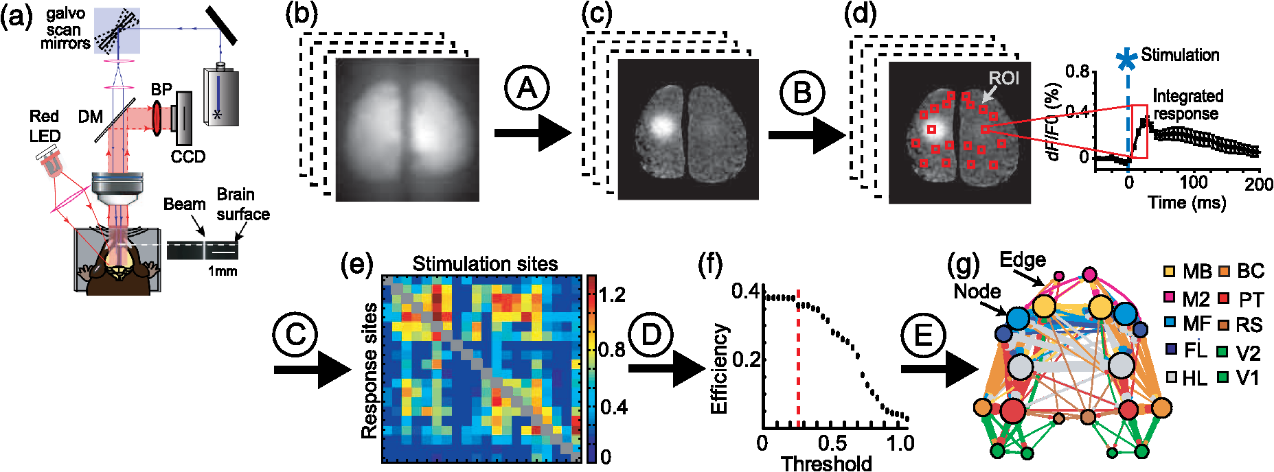

4. Optical Imaging and Network Analysis

4.1.

Voltage-Sensitive-Dye Imaging

ChR2 transgenic mice were obtained from the Jackson Laboratory [line 18, stock 007612, strain B6.Cg-Tg (Thy1-COP4/EYFP) 18Gfng/J]. All experiments were conducted with approval from the University of British Columbia Animal Care Committee and in accordance with guidelines set forth by the Canadian Council for Animal Care. At approximately 16 weeks of age, transgenic ChR2 mice²⁷ were anesthetized with isoflurane (1.0%), and given a large bilateral craniotomy ( $8 \times 8 mm$ ). To minimize any movement artifacts in the image acquisition, the skull was fastened to a custom-designed steel plate with dental cement. This steel plate was screwed onto a metal baseplate that could be mounted onto the imaging rig for mechanically stable imaging.²⁸ Following the craniotomy, we used a blue-shifted VSD, RH1962 (Optical Imaging, New York),²⁹ dissolved in 4-(2-hydroxyethyl)-1-piperazineethanesulfonic acid (HEPES)-buffered saline solution to an optical density of 5 to 7, measured at 550 nm. The dye was applied to the exposed cortex for 60 to 90 min in order to stain all cortical layers.³⁰ The brain was then washed with HEPES-buffered saline solution to remove any unloaded dye, covered with 1.5% agarose (made in HEPES-buffered saline) and sealed with a glass coverslip to minimize movement artifacts due to respiration. VSD imaging followed immediately.

For VSD data collection, 12-bit images were captured with 6.67-ms exposure using a CCD camera (1M60 Pantera, Dalsa, Waterloo, Ontario, Canada), and EPIX E4DB frame grabber with XCAP 3.7 imaging software (EPIX, Inc., Buffalo Grove, Illinois). VSD was excited with a red LED (Luxeon K2, 627 nm centre) and the camera focused 400 μm below the surface to prevent VSD signal distortion from large surface vessels. VSD fluorescence was filtered using a 673 to 703 nm bandpass filter (Semrock New York), after reflection by a dichroic mirror (510 dcspxr; 400 to 495 transmission reflection 550 to 725 nm, Chroma, Bellows Falls, Vermont). Images were taken through a macroscope consisting of coupled camera lenses (Nikon NIKKOR $f = 35 mm$ and $f = 50 mm$ ) ( $8.4 \times 8.4 mm$ field of view, $65 μ m$ per pixel). The depth of field was 1.20 mm and was defined by the distance along the optical axis where the resolution was better than 10 lines per mm, corresponding to a maximum blur of 2 pixels.

For each trial, either sensory or optogenetic stimulation was performed, as described in Secs. 4.2 and 4.3. For all types of stimulation, images were collected for 205 ms before stimulation and 515 ms after stimulation for a total of 108 frames at 150 Hz ( $6.67 ms / frame$ ). To correct for dye bleaching over time, stimulation trials were divided by null stimulation trials. Null stimulation trials were interleaved with stimulation trials to correct for any dye bleaching that may take place over the course of the experiment (for every two stimulation trials, there was one null stimulation trial). To reduce the impact of spontaneous cortical activity,²⁵ we averaged 2 to 10 trials of stimulus presentation per stimulation type. VSD responses were expressed as a percent change relative to baseline VSD fluorescence ( $Δ F / F_{0} \times 100 %$ ).

4.2.

Sensory Stimulation

We used sensory stimuli to locate the functional sites of the primary sensory cortical areas. Specifically, we mapped the hindlimb, forelimb, C2 whisker, and visual system. Probes were inserted subcutaneously to each of the paws and a 1 ms, 1-mA pulse was delivered to locate the functional forelimb and hindlimb areas of the primary somatosensory cortex (FL and HL, respectively). A piezo device was attached to a single whisker (C2) to locate the somatosensory barrel cortex (BC). A combined blue and green LED light stimulus was presented to map the primary visual cortex (V1). These functional sites were then used as the coordinates for the photostimulation sites and to stereotaxically locate secondary and association areas for photostimulation.

4.3.

Optogenetic Stimulation

We used transgenic ChR2 mice from Jackson Laboratory [line 18, stock 007612, strain B6.Cg-Tg (Thy1-COP4/EYFP) 18Gfng/J]. These mice express ChR2 in layer V neurons,²⁷ allowing for optogenetic photostimulation at any area of the cortex. We used a 473-nm diode pumped solid-state laser (CNI Optoelectronics, Changhun, China) and a 1-ms, 5-mW pulse to stimulate these ChR2-expressing neurons. In order to verify that the beam was relatively collimated, we imaged the beam profile as it passed through a cuvette containing a fluorescein solution. The FWHM at the top of the cuvette was $68 μ m$ and has an $f$ -number of 34. This degree of collimation reduced the potential effects of differences in path length due to brain curvature.

The beam was positioned on the cortex using custom-written software in IGOR PRO (Portland, Oregon) which controlled galvanometer scan mirrors (Cambridge Tech, Lexington, Massachusetts), via analog output voltage from PCI-6115 DAQ (National Instruments, Austin, Texas). The IGOR program controlled the timing of each stimulation trial with TTL triggers to XCAP from a second DAQ (PCI-6036E). The stimulation delay (205 ms) and pulse length (a single 1-ms pulse) were controlled by an A–M Systems (Sequim, Washington) isolated pulse stimulator. The intensity and duration of the photostimulation was chosen based on its ability to reliably evoke electroencephalogram (EEG) responses in a ChR2 mouse. We determined 20 regions of interest (ROIs) that we used for photostimulation sites (10 per hemisphere): secondary motor cortex (M2), primary motor cortex (MB), forelimb area of the primary motor cortex (MF), forelimb area of the primary somatosensory cortex (FL), hindlimb area of the primary somatosensory cortex (HL), barrel cortex of the primary somatosensory cortex (BC), parietal cortex (PT), retrosplenial cortex (RS), secondary visual cortex (V2), and primary visual cortex (V1). These sites were calculated per animal, and were based on known sensory coordinates (primary sensory areas were functionally mapped from sensory stimulation, as described previously) and on stereotaxic coordinates.³¹ (Note: the coordinates for these 20 ROIs can be found with the MATLAB^® code on our website. These ROIs are listed according to pixel location, given our $128 \times 128$ pixel images. See file: “pos.mat.”) Photostimulation was given in a semirandom, interleaved order to reduce the possibility of sequential stimulation at neighboring cortical sites and to reduce any time-dependent effects of anesthesia depth or cortical excitability. There was a 10-s interval between trials to allow for VSD fluorescence to fully recover.

4.4.

Data Analysis in MATLAB^®

VSD responses to stimulation were captured using EPIX software (see sample data on our website) and then processed offline using custom-written MATLAB^® code (see sample code, “NetworkAnalysis_VSD.m,” on our website). To correct for VSD bleaching over the imaging time, the VSD response was normalized by dividing by the VSD response to a null stimulation trial, for example NOA.tif. VSD responses were then calculated and expressed as a percent change relative to baseline VSD fluorescence ( $Δ F / F_{0} \times 100 %$ ). For each stimulation, we averaged 2 to 10 trials together to create an average VSD response; for example, two trials of stimulation of the left forelimb somatosensory cortex: FLL1.tif and FLL2.tif. Images were spatially filtered with a Gaussian kernel 2-d filter (sigma 2.5). (See code ”NetworkAnalysis_VSD.m”—Section A.)

Integrated VSD responses were quantified at the same 20 ROIs that were used as photostimulation sites. Each response area measured $5 \times 5$ pixels, or $0.0625 {mm}^{2}$ , and responses were taken at a number of time points after stimulation (6, 12, and 20 ms after stimulation). Therefore, for each photostimulation site, VSD responses were collected from the remaining 19 sites. Responses were not taken from the photostimulation site due to transient photobleaching caused by the laser. In order to ensure that the VSD responses we collected were not simply due to noise, we excluded any VSD responses that were less than 2.5 times greater than the standard deviation of the baseline. Responses that did not meet this threshold were assigned a value of zero. (See code “NetworkAnalysis_VSD.m”—Section B. Note that for simplicity, this code calculates responses at a single time point only.)

In a given connectivity matrix, the number of rows or number of columns is equal to the number of nodes in the network, while the elements within the matrix represent the edges within the network. Here, VSD responses were put into a $20 \times 20$ weighted matrix, arranged with photostimulation sites on the $x$ axis, and response sites on the $y$ axis, with the integrated VSD response as the elements of the matrix. For each node, the connectivity matrix shows in-strength as the rows (the strength of the connections coming to the node when other areas were photostimulated) and out-strength as the columns (the strength of the connections to other areas when the node was photostimulated). We chose to represent the data as a weighted, directed network to preserve the information regarding reciprocal connections and their relative importance (as opposed to a binary, undirected network which would simply indicate the presence or absence of an edge between nodes, but would not provide any information on the direction of information processing or the strength of that connection). This allows us to make the distinction between incoming and outgoing strength as well as the relative importance of each node to the network as a whole. We chose to order our connectivity matrix by approximate anatomical ROI position, from anterior to posterior in the left hemisphere, and then anterior to posterior in the right hemisphere: M2L, MBL, MFL, FLL, HLL, BCL, PTL, RSL, V2L, V1L, M2R, MBR, MFR, FLR, HLR, BCR, PTR, RSR, V2R, V1R. This makes it easier to distinguish clusters of activity in neighboring nodes; for example, the top-left quadrant of the connectivity matrix shows strong VSD responses in the left hemisphere somatosensory areas after left hemisphere photostimulation of the somatosensory areas. Note that the order of the nodes does not affect the computation of network measures but is important for visualization of the connectivity matrix and the network diagram. (See “NetworkAnalysis_VSD.m” code—Section C.)

We chose to focus on the 20 ms poststimulation time point based on previous work that showed the greatest VSD activation,¹⁶ however, these analyses can easily be applied to a different time point or a different set of ROIs.

4.5.

Network Analysis in MATLAB^®

Once the data is arranged in a connectivity matrix, it is possible to use functions from the Brain Connectivity Toolbox¹⁵^,³² for network analysis. The Brain Connectivity Toolbox has a number of functions for both directed and undirected networks, weighted and unweighted networks (for a full review of these functions and network properties, see Ref. 15). We used the Brain Connectivity Toolbox to determine a suitable threshold for creating network diagrams (see Sec. 4.6) and calculate various network properties (see Appendix). Network analysis may be used to describe global network properties such as characteristic path length and efficiency (Table 1), or may be used to describe properties per node, such as node degree and node strength (Table 2). For simplicity, only results for three example nodes are shown for a single animal. Given that this a single animal example, left and right hemisphere differences are unlikely to represent a true lateralization of function, but rather some noise within the system.

Table 1

Global network properties calculated with the Brain Connectivity Toolbox.

Global network property	Unthresholded network	Thresholded network (0.2577)	Difference (%)
Number of connections	231	158	$- 31.6$
Characteristic path length	3.35	2.72	$- 18.8$
Global efficiency	0.38	0.36	$- 5.3$

Table 2

Example per-node network properties calculated with the Brain Connectivity Toolbox (network thresholded at 0.2257).

Node	Node degree	Node strength	Mean strength per edge	Betweenness centrality
HLL	22	15.1	0.69	6
PTL	23	14.1	0.61	22
V2L	4	1.8	0.45	0
HLR	21	12.9	0.61	8
PTR	19	10.3	0.54	35
V2R	0	0	–	0

4.6.

Network Diagram Generation in MATLAB^®

Once a square connectivity matrix has been generated, it is possible to use the bioinformatics toolbox in MATLAB^® to generate network diagrams. This toolbox includes functions and methods for creating, visualizing, and manipulating graph data as a directed network. Here, nodes may represent proteins, genes, locations, or brain regions and edges may represent interactions, dependencies, or connections (structural or functional). Importantly, the graph visualization function in the bioinformatics toolbox does not work with nonsquare matrices. Using the biograph function in MATLAB^®, the network diagram can be formatted to change the position of the nodes to match an anatomical representation, or to change properties of the elements within the diagram (for example, if a weighted connectivity matrix is being used, node size can be made to be proportional to the strength of the connection weight).

The network diagrams that we use here are simply a graphical representation of the information in the connectivity matrix; however, these diagrams are useful to illustrate the data. In order to keep the network diagram illustration relatively simple, we chose to display only the strongest connections in the network by applying a consistent threshold across the connectivity matrix. This threshold was applied for display purposes only, as it was difficult to visually assess trends within the diagram of the unthresholded network due to the large number of connections present. To determine the threshold, we examined the effects of various threshold levels on common global network properties, including characteristic path length and efficiency [see Fig. 2(d)] using functions from the Brain Connectivity Toolbox.¹⁵ (See “NetworkAnalysis_VSD.m” code—Section D and see Table 1.) An ideal threshold will remove a large number of connections without having a severe effect on global network properties. This generally allows for easier visualization of the most important connections within the network. In our previous studies,¹²^,¹⁶ we limited the use of thresholded network to visualization only, and performed all statistical analyses with the unthresholded network. The suitability of the thresholded network for further analysis should be carefully considered for the particular system under study.

Once we had a thresholded square matrix (connections that did not reach the threshold level were given a value of zero), we used the biograph function in MATLAB^® to visualize the graph. Using this function, it is possible to identify the nodes with identification strings and color code them. While the biograph function will automatically arrange the nodes in space, we defined the placement of our nodes according to the stereotaxic coordinates we mapped during each experiment so the positions of the nodes were anatomically relevant.¹²^,¹⁶ We used the out-strength of the node (that is, the sum of the outgoing connections) to determine the overall size of the node within our graph. Similarly, we used the weight of the connection strength between two given nodes to determine the thickness of the edge connecting these two nodes. Edges were also color-coordinated to match the node from which the connection was coming (out-strength). This generated network diagrams that had the nodes in the correct stereotaxic position, with the node size relating to the total node out-strength, and with edges relating to weighted connection strength (in this case, integrated VSD response), and color-coded by node. (See “NetworkAnalysis_VSD.m” code—Section E).

5. Caveats and Limitations of Network Analysis

Due to the nature of our preparation, one of the biggest limitations is that VSD imaging is only capable of measuring surface cortical connections, and cannot be used for subcortical connections or provide depth information about cortical connections. Thus, our networks only represent intracortical connections, although it is possible that there are subcortical contributions (especially when considering the VSD response at later time points). Despite the fact that we cannot account for possible subcortical contribution using our method, it is still possible to use network analysis to examine directionality and relative node strength within the cortical network. For example, we have demonstrated that the strength of reciprocal intracortical connections between primary and secondary areas are unequal, suggesting different roles in information processing between these nodes.¹⁶ When identifying hub nodes using betweenness centrality, it is important to recognize that there may be contributions from areas outside the scope of the measured network. A high betweenness centrality may therefore also reflect strong connections through an inaccessible hub; for example, a subcortical area or even a cortical area outside of the imaging window.

While we cannot distinguish between cortical and subcortical contribution with VSD imaging, this distinction could be made using a different technique, such as fMRI. Indeed, optogenetic stimulation has been paired with fMRI in order to map whole brain networks.³³^–³⁵ However, the disadvantage of using fMRI is that signals are much slower compared to VSD imaging, and the fMRI signal and its relationship to neuronal coupling is not always clear.³⁶ Each mapping technique will have strengths and limitations with respect to network analysis, thus, results from network analysis should be interpreted with the technique in mind.

One of the general challenges in applying network analysis is determining how to define nodes.³⁷^,³⁸ The parcellation of the brain into different nodes should be done such that there is no overlap between nodes (that is, each node should be separate from the others). In experimental studies, nodes may be defined by the cytoarchitecture of the tissue (for example, motor cortex can be defined by the absence of layer IV cells), by the functionality of the tissue (for example, motor cortex can be mapped by the region that is active during the execution of a motor task), or by previously defined stereotactic coordinates (for example, using a brain atlas). It is important for the parcellation scheme to be consistent between studies to allow for contrast and comparison.³⁷ Here, we determined nodes on the functional VSD responses to sensory stimulation (for the primary sensory areas) and on stereotaxic coordinates. Functional maps were completed for each animal to account for any animal-to-animal variability in cortical map distribution.

Detecting network connectivity abnormalities in neuropsychiatric disorders¹^,³⁹^,⁴⁰ or brain injury⁹ may prove to be useful in understanding these conditions. Particularly, it may be useful to relate structural and functional networks. However, one of the challenges with comparing brain networks is differences in edge density—for example, functional brain networks may be denser than anatomical networks due to numerous redundant connections between areas not directly anatomically connected.¹⁵^,⁴¹ As anatomical mapping efforts continue and more detailed structural maps become available, it will be easier to draw comparisons between functional and anatomical networks.¹^,¹⁵ While structural and functional maps do not always correlate, the mouse dorsal cortex does offer the ability to correlate functional and structural connections.²⁵

6. Prospects

Regional, functional connectomics by network analysis holds great potential for the interpretation of neuroimaging data at multiple scales of organization. Using these analyses, we can further investigate cortical organization in the healthy and unhealthy brain. For instance, network changes may be useful in tracking progressive disease models, such as Alzheimer’s disease,⁴² and may lead to better preventative treatment methods. Network analysis may also prove useful in tracking recovery of brain function after brain injury, such as stroke,¹⁸ or could be used to inform future studies about which areas of the brain are most vulnerable to damage; for example, damage to hub areas will have great effects on the whole network.⁴³ The connectomics approach may prove especially useful in the clinical setting where noninvasive imaging techniques such as fMRI can collect data relatively easily (for example, the collection of spontaneous fMRI data requires little effort on behalf of the patient) and over multiple time points.¹¹

Future studies using animal models may take advantage of recently developed sensors, which would allow for more specific imaging of the network. While the VSD signal includes contribution from excitatory and inhibitory cells,⁴⁴ tools such as genetically encoded calcium imaging could be used to investigate specific aspects of the neuronal signal.²⁴^,⁴⁵ Novel voltage-sensitive fluorescent proteins (VSFPs) could also be used to investigate networks over time (for example, several time points in the poststroke period could be investigated in the same animal using VSFPs), and could be used to investigate cell-specific, layer-specific contributions to the signal.⁴⁵

Acknowledgments

This work was supported by the Canadian Institutes of Health Research (CIHR Operating Grant MOP-111009), the Heart and Stroke Foundation of Canada (grant in aid), and the Canadian Partnership for Stroke Recovery expansion.

Appendices

Appendix

The typically observed brain network can be considered as a small-world network. This type of network has efficient information transfer with minimal wiring costs, has both local processing (specialization) and global processing (integration), and is resistant to random network damage.¹ Abnormal or pathological networks do not necessarily have these characteristics. In cases where networks are altered due to increased aberrant connectivity,¹^,³⁹^,⁴⁰ there may be increased clustering, decreased characteristic path lengths, and increased efficiency. For the purposes of this review, we describe network properties in the Appendix in the context of the typical brain network.

A1.

Basic Properties in Network Analysis

A1.1.

Degree

The degree is a measure of the number of links connected to a node and broadly reflects the importance of the node within the network; nodes with more links have a higher degree, and nodes with fewer links have a lower degree. In a directed network, degree is the sum of the incoming (afferent) and outgoing (efferent) connections in a given node. Degree can be broken down into in-degree and out-degree (corresponding to the sum of incoming and sum of outgoing connections for a give node, respectively). The comparison of in-degree and out-degree can be useful in describing the properties of the node. A node with high in-degree can be considered an integrator, whereas a node with a high out-degree can be seen as distributors.⁴⁶

The degree distribution is the probability distribution describing the likelihood of a given node having a given degree.⁴⁷ Degree distribution may be used to compare and classify network types: for example, brain networks tend to have a non-Gaussian degree distribution, while a random network has a Gaussian degree distribution.¹

A1.2.

Clustering Coefficient

For a given node, $X$ , all nodes that have a direct projection to this node, and all nodes to which $X$ has a direct projection, are considered neighbors. Connectivity between neighbors is used to determine clustering. The presence of clusters, or groups, can represent the ability for specialized processing to occur within the network and is calculated using the clustering coefficient, which measures the fraction of the node’s neighbors that are also neighbors to each other.⁴⁸ This determines how much clustered connectivity takes place around an individual node. In a random network (where node pairs are connected randomly by a probability, $p$ ), there would be relatively low clustering; however, many real-life complex networks show a high degree of clustering, which may be indicative of specialization.²²

A1.3.

Characteristic Path Length

The distance between two nodes in a network is defined as the number of edges along the shortest path connecting the two nodes (that is, the lowest number of connections possible between the pair of nodes). The characteristic path length is the mean distance of the shortest path between two given nodes in a network, averaged over all pairs of nodes.⁴⁸ Characteristic path length gives a measure of network integration. Shorter average path length typically suggests fast communication within the network.³⁹ The characteristic path length of most real, complex networks is relatively small, allowing for the efficient transfer of information between specialized regions.⁴⁸

A1.4.

Efficiency

Efficiency is a measure of integration or information processing within the network. Global efficiency is the average inverse shortest path length in the network.⁴⁹ High efficiency and relatively low wiring cost (number of connections) are important features of small-world networks.⁵⁰

A1.5.

Betweenness Centrality

The betweenness centrality is a measure of the number of shortest paths that pass through a given node.⁵¹ A higher centrality indicates a “hub” node, meaning that the node has many important connections for information transfer within the network. Nodes with a high betweenness centrality are highly important for network efficiency and integration. Hub nodes are a characteristic of small-world networks, and are often seen in real, complex networks. Networks containing hub nodes tend to be resistant to random network damage but are vulnerable to targeted damage of these hub nodes.⁴³

For a full description of network properties, see Ref. 15.

References

1.

E. Bullmore and O. Sporns, “Complex brain networks: graph theoretical analysis of structural and functional systems,” Nat. Rev. Neurosci., 10 (3), 186 –198 (2009). http://dx.doi.org/10.1038/nrn2575 NRNAAN 1471-0048 Google Scholar

2.

O. Sporns, G. Tononi and R. Kotter, “The human connectome: a structural description of the human brain,” PLoS Comput. Biol., 1 (4), e42 (2005). http://dx.doi.org/10.1371/journal.pcbi.0010042 PCBLBG 1553-734X Google Scholar

3.

E. S. Lein et al., “Genome-wide atlas of gene expression in the adult mouse brain,” Nature, 445 (7124), 168 –176 (2007). http://dx.doi.org/10.1038/nature05453 NATUAS 0028-0836 Google Scholar

4.

S. W. Oh et al., “A mesoscale connectome of the mouse brain,” Nature, 508 (7495), 207 –214 (2014). http://dx.doi.org/10.1038/nature13186 NATUAS 0028-0836 Google Scholar

5.

J. W. Bohland et al., “A proposal for a coordinated effort for the determination of brainwide neuroanatomical connectivity in model organisms at a mesoscopic scale,” PLoS Comput. Biol., 5 (3), e1000334 (2009). http://dx.doi.org/10.1371/journal.pcbi.1000334 PCBLBG 1553-734X Google Scholar

6.

B. Zingg et al., “Neural networks of the mouse neocortex,” Cell, 156 (5), 1096 –1111 (2014). http://dx.doi.org/10.1016/j.cell.2014.02.023 CELLB5 0092-8674 Google Scholar

7.

T. Hjornevik et al., “Three-dimensional atlas system for mouse and rat brain imaging data,” Front Neuroinf., 1 (4), 1 –11 (2007). http://dx.doi.org/10.3389/neuro.11.004.2007 1662-5196 Google Scholar

8.

G. Silasi and T. H. Murphy, “Stroke and the connectome: how connectivity guides therapeutic intervention,” Neuron, 83 (6), 1354 –1368 (2014). http://dx.doi.org/10.1016/j.neuron.2014.08.052 NERNET 0896-6273 Google Scholar

9.

L. Cheng et al., “Reorganization of functional brain networks during the recovery of stroke: a functional MRI study,” in Proc. Conf. IEEE Engineering in Medicine and Biology Society, 4132 –4135 (2012). Google Scholar

10.

S. Feldt, P. Bonifazi and R. Cossart, “Dissecting functional connectivity of neuronal microcircuits: experimental and theoretical insights,” Trends Neurosci., 34 (5), 225 –236 (2011). http://dx.doi.org/10.1016/j.tins.2011.02.007 TNSCDR 0166-2236 Google Scholar

11.

M. P. van den Heuvel and H. E. Hulshoff Pol, “Exploring the brain network: a review on resting-state fMRI functional connectivity,” Eur. Neuropsychopharmacol., 20 (8), 519 –534 (2010). http://dx.doi.org/10.1016/j.euroneuro.2010.03.008 EURNE8 0924-977X Google Scholar

12.

D. H. Lim et al., “Optogenetic mapping after stroke reveals network-wide scaling of functional connections and heterogeneous recovery of the peri-infarct,” J. Neurosci., 34 (49), 16455 –16466 (2014). http://dx.doi.org/10.1523/JNEUROSCI.3384-14.2014 JNRSDS 0270-6474 Google Scholar

13.

W. M. Otte et al., “Effects of transient unilateral functional brain disruption on global neural network status in rats: a methods paper,” Front. Syst. Neurosci., 8 1 –409 (2014). http://dx.doi.org/10.3389/fnsys.2014.00040 FSNRAR 1662-5137 Google Scholar

14.

D. H. Lim, J. M. LeDue and T. H. Murphy, “Neurophotonics tutorial on making connectivity diagrams from Channelrhodopsin-2 stimulated data,” (2015) http://www.neuroscience.ubc.ca/faculty/murphy_software.html Google Scholar

15.

M. Rubinov and O. Sporns, “Complex network measures of brain connectivity: uses and interpretations,” Neuroimage, 52 (3), 1059 –1069 (2010). http://dx.doi.org/10.1016/j.neuroimage.2009.10.003 NEIMEF 1053-8119 Google Scholar

16.

D. H. Lim et al., “In vivo large-scale cortical mapping using channelrhodopsin-2 stimulation in transgenic mice reveals asymmetric and reciprocal relationships between cortical areas,” Front. Neural Circuits, 6 (11), 1 –19 (2012). http://dx.doi.org/10.3389/fncir.2012.00011 FNCRA5 1662-5110 Google Scholar

17.

A. L. Wheeler et al., “Identification of a functional connectome for long-term fear memory in mice,” PLoS Comput. Biol., 9 (1), e1002853 (2013). http://dx.doi.org/10.1371/journal.pcbi.1002853 PCBLBG 1553-734X Google Scholar

18.

C. Grefkes and G. R. Fink, “Reorganization of cerebral networks after stroke: new insights from neuroimaging with connectivity approaches,” Brain, 134 (5), 1264 –1276 (2011). http://dx.doi.org/10.1093/brain/awr033 BRAIAK 0006-8950 Google Scholar

19.

M. P. van Meer et al., “Extent of bilateral neuronal network reorganization and functional recovery in relation to stroke severity,” J. Neurosci., 32 (13), 4495 –4507 (2012). http://dx.doi.org/10.1523/JNEUROSCI.3662-11.2012 JNRSDS 0270-6474 Google Scholar

20.

M. P. van den Heuvel et al., “Aberrant frontal and temporal complex network structure in schizophrenia: a graph theoretical analysis,” J. Neurosci., 30 (47), 15915 –15926 (2010). http://dx.doi.org/10.1523/JNEUROSCI.2874-10.2010 JNRSDS 0270-6474 Google Scholar

21.

S. Qiu et al., “Circuit-specific intracortical hyperconnectivity in mice with deletion of the autism-associated Met receptor tyrosine kinase,” J. Neurosci., 31 (15), 5855 –5864 (2011). http://dx.doi.org/10.1523/JNEUROSCI.6569-10.2011 JNRSDS 0270-6474 Google Scholar

22.

O. Sporns et al., “Organization, development and function of complex brain networks,” Trends Cognit. Sci., 8 (9), 418 –425 (2004). http://dx.doi.org/10.1016/j.tics.2004.07.008 TCSCFK 1364-6613 Google Scholar

23.

A. Roebroeck, E. Formisano and R. Goebel, “Mapping directed influence over the brain using Granger causality and fMRI,” Neuroimage, 25 (1), 230 –242 (2005). http://dx.doi.org/10.1016/j.neuroimage.2004.11.017 NEIMEF 1053-8119 Google Scholar

24.

J. P. Rickgauer, K. Deisseroth and D. W. Tank, “Simultaneous cellular-resolution optical perturbation and imaging of place cell firing fields,” Nat. Neurosci., 17 (12), 1816 –1824 (2014). http://dx.doi.org/10.1038/nn.3866 NANEFN 1097-6256 Google Scholar

25.

M. H. Mohajerani et al., “Spontaneous cortical activity alternates between motifs defined by regional axonal projections,” Nat. Neurosci., 16 (10), 1426 –1435 (2013). http://dx.doi.org/10.1038/nn.3499 NANEFN 1097-6256 Google Scholar

26.

M. P. van Meer et al., “Recovery of sensorimotor function after experimental stroke correlates with restoration of resting-state interhemispheric functional connectivity,” J. Neurosci., 30 (11), 3964 –3972 (2010). http://dx.doi.org/10.1523/JNEUROSCI.5709-09.2010 JNRSDS 0270-6474 Google Scholar

27.

B. R. Arenkiel et al., “In vivo light-induced activation of neural circuitry in transgenic mice expressing channelrhodopsin-2,” Neuron, 54 (2), 205 –218 (2007). http://dx.doi.org/10.1016/j.neuron.2007.03.005 NERNET 0896-6273 Google Scholar

28.

T. C. Harrison, A. Sigler and T. H. Murphy, “Simple and cost-effective hardware and software for functional brain mapping using intrinsic optical signal imaging,” J. Neurosci. Methods, 182 (2), 211 –218 (2009). http://dx.doi.org/10.1016/j.jneumeth.2009.06.021 JNMEDT 0165-0270 Google Scholar

29.

D. Shoham et al., “Imaging cortical dynamics at high spatial and temporal resolution with novel blue voltage-sensitive dyes,” Neuron, 24 (4), 791 –802 (1999). http://dx.doi.org/10.1016/S0896-6273(00)81027-2 NERNET 0896-6273 Google Scholar

30.

M. H. Mohajerani et al., “Mirrored bilateral slow-wave cortical activity within local circuits revealed by fast bihemispheric voltage-sensitive dye imaging in anesthetized and awake mice,” J. Neurosci., 30 (10), 3745 –3751 (2010). http://dx.doi.org/10.1523/JNEUROSCI.6437-09.2010 JNRSDS 0270-6474 Google Scholar

31.

G. Paxinos and K. B. Franklin, The Mouse Brain in Stereotaxic Coordinates, Academic Press, San Diego (2001). Google Scholar

32.

M. Rubinov and O. Sporns, “Brain Connectivity Toolbox,” (2015) http://www.brain-connectivity-toolbox.net Google Scholar

33.

M. Desai et al., “Mapping brain networks in awake mice using combined optical neural control and fMRI,” J. Neurophysiol., 105 (3), 1393 –1405 (2011). http://dx.doi.org/10.1152/jn.00828.2010 JONEA4 0022-3077 Google Scholar

34.

I. Kahn et al., “Characterization of the functional MRI response temporal linearity via optical control of neocortical pyramidal neurons,” J. Neurosci., 31 (42), 15086 –15091 (2011). http://dx.doi.org/10.1523/JNEUROSCI.0007-11.2011 JNRSDS 0270-6474 Google Scholar

35.

J. H. Lee et al., “Global and local fMRI signals driven by neurons defined optogenetically by type and wiring,” Nature, 465 (7299), 788 –792 (2010). http://dx.doi.org/10.1038/nature09108 NATUAS 0028-0836 Google Scholar

36.

N. K. Logothetis, “What we can do and what we cannot do with fMRI,” Nature, 453 (7197), 869 –878 (2008). http://dx.doi.org/10.1038/nature06976 NATUAS 0028-0836 Google Scholar

37.

J. Wang et al., “Parcellation-dependent small-world brain functional networks: a resting-state fMRI study,” Hum. Brain Mapp., 30 (5), 1511 –1523 (2009). http://dx.doi.org/10.1002/hbm.v30:5 HBRME7 1065-9471 Google Scholar

38.

B. R. White et al., “Imaging of functional connectivity in the mouse brain,” PLoS One, 6 (1), e16322 (2011). http://dx.doi.org/10.1371/journal.pone.0016322 1932-6203 Google Scholar

39.

M. A. Kramer and S. S. Cash, “Epilepsy as a disorder of cortical network organization,” Neuroscientist, 18 (4), 360 –372 (2012). http://dx.doi.org/10.1177/1073858411422754 NROSFJ 1073-8584 Google Scholar

40.

J. C. Reijneveld et al., “The application of graph theoretical analysis to complex networks in the brain,” Clin. Neurophysiol., 118 (11), 2317 –2331 (2007). http://dx.doi.org/10.1016/j.clinph.2007.08.010 CNEUFU 1388-2457 Google Scholar

41.

J. S. Damoiseaux and M. D. Greicius, “Greater than the sum of its parts: a review of studies combining structural connectivity and resting-state functional connectivity,” Brain Struct. Funct., 213 (6), 525 –533 (2009). http://dx.doi.org/10.1007/s00429-009-0208-6 BSFRCD 1863-2653 Google Scholar

42.

W. de Haan et al., “Functional neural network analysis in frontotemporal dementia and Alzheimer’s disease using EEG and graph theory,” BMC Neurosci., 10 (101), 1 –12 (2009). http://dx.doi.org/10.1186/1471-2202-10-101 BNMEA6 1471-2202 Google Scholar

43.

O. Sporns, C. J. Honey and R. Kotter, “Identification and classification of hubs in brain networks,” PLoS One, 2 (10), e1049 (2007). http://dx.doi.org/10.1371/journal.pone.0001049 1932-6203 Google Scholar

44.

A. Grinvald and R. Hildesheim, “VSDI: a new era in functional imaging of cortical dynamics,” Nat. Rev. Neurosci., 5 (11), 874 –885 (2004). http://dx.doi.org/10.1038/nrn1536 NRNAAN 1471-0048 Google Scholar

45.

M. Scanziani and M. Hausser, “Electrophysiology in the age of light,” Nature, 461 (7266), 930 –939 (2009). http://dx.doi.org/10.1038/nature08540 NATUAS 0028-0836 Google Scholar

46.

M. Kaiser, “A tutorial in connectome analysis: topological and spatial features of brain networks,” Neuroimage, 57 (3), 892 –907 (2011). http://dx.doi.org/10.1016/j.neuroimage.2011.05.025 NEIMEF 1053-8119 Google Scholar

47.

A. L. Barabasi and R. Albert, “Emergence of scaling in random networks,” Science, 286 (5439), 509 –512 (1999). http://dx.doi.org/10.1126/science.286.5439.509 SCIEAS 0036-8075 Google Scholar

48.

D. J. Watts and S. H. Strogatz, “Collective dynamics of ‘small-world’ networks,” Nature, 393 (6684), 440 –442 (1998). http://dx.doi.org/10.1038/30918 NATUAS 0028-0836 Google Scholar

49.

V. Latora and M. Marchiori, “Efficient behavior of small-world networks,” Phys. Rev. Lett., 87 (19), 198701 (2001). http://dx.doi.org/10.1103/PhysRevLett.87.198701 PRLTAO 0031-9007 Google Scholar

50.

S. Achard and E. Bullmore, “Efficiency and cost of economical brain functional networks,” PLoS Comput. Biol., 3 (2), e17 (2007). http://dx.doi.org/10.1371/journal.pcbi.0030017 PCBLBG 1553-734X Google Scholar

51.

L. C. Freeman, “Centrality in social networks: conceptual clarification,” Soc. Networks, 1 (3), 215 –239 (1979). http://dx.doi.org/10.1016/0378-8733(78)90021-7 0378-8733 Google Scholar

Biographies for the authors are not available.

CC BY: © The Authors. Published by SPIE under a Creative Commons Attribution 4.0 Unported License. Distribution or reproduction of this work in whole or in part requires full attribution of the original publication, including its DOI.

Citation Download Citation

Diana H. Lim, Jeffrey M. LeDue, and Timothy H. Murphy "Network analysis of mesoscale optical recordings to assess regional, functional connectivity," Neurophotonics 2(4), 041405 (22 June 2015). https://doi.org/10.1117/1.NPh.2.4.041405

Published: 22 June 2015

Access the abstract

JOURNAL ARTICLE
8 PAGES

DOWNLOAD PAPER SAVE TO MY LIBRARY

GET CITATION

CITATIONS

Cited by 18 scholarly publications.

Explore citations on Lens.org

KEYWORDS

Network security

Brain

Neuroimaging

Optical imaging

Sensors

Photostimulation

Optical recording

1.

Introduction

2.

Why Use Network Analysis?

3.

Basic Concepts in Network Analysis