

|
|
1.IntroductionFunctional near-infrared spectroscopy (fNIRS) is an optical technique that uses near-infrared light to monitor cortical functional activation. Human tissues are relatively transparent to light in the near-infrared range where the dominant absorbers are oxygenated (HbO) and deoxygenated (HbR) hemoglobin. As these two chromophores have significantly different absorption spectra, the changes in the intensity of light emitted by a source placed on a subject’s scalp and backscattered to a detector located at a distance of several centimeters can be used to recover the changes in HbO and HbR concentration occurring in the cerebral cortex.1,2 The interaction between near-infrared light and biological tissue is dominated by optical scattering.2 As a result, the path traveled by near-infrared photons in tissue resembles a random walk. The fluence distribution produced by a source transmitting light into such highly scattering media can be determined using a range of numerical methods, including the finite-element method, (which discretizes the diffusion approximation to the radiative transfer equation into mesh elements3) and more explicit Monte-Carlo simulation approaches.4,5 By taking the element-wise product of the fluence distribution of the source with the adjoint fluence distribution of the detector modeled as a source, the photon measurement density function (PMDF) can be calculated. This distribution gives the probability of the detected near-infrared light traveling through a given region of tissue, which can also be thought of as how sensitive the fNIRS measurement will be to changes in chromophore concentration in that region of tissue. Increasing the distance between the source and detector of near-infrared light will generally increase the proportion of detected photons that have traveled through deeper tissues, thus increasing the sensitivity of that channel to the brain. However, this increase in sensitivity to deeper tissues is at the expense of a lower signal-to-noise ratio (SNR) in the measured signal,6 simply because fewer photons will make it to the detector, per unit time, without being absorbed. It has been shown that, for the adult population, a source–detector distance of 30 mm is a good compromise between providing reasonable sensitivity to the cortex and enough detected light to provide an acceptable SNR.7,8 In the infant population, due to the thinner scalp and skull, the typical fNIRS source–detector distance is 20 or 25 mm.9,10 The human scalp and skull tissues are highly vascularized and their mean total thickness in the adult head is .11 Light traveling from a source to a detector must pass through these layers twice. As a result, fNIRS measurements are highly sensitive to scalp and skull tissues; in fact, fNIRS measurements are significantly more sensitive to these superficial layers than they are to the brain.12 This means that the signal measured by standard fNIRS channels contains the effect of hemoglobin concentration changes occurring not only in the brain, but also in scalp and skull tissues. This contamination of the fNIRS signal with superficial hemodynamic fluctuations is a well-known problem in the fNIRS field and remains one of the biggest challenges for fNIRS technology.13–15 Fluctuations in HbO and HbR concentrations in the superficial tissues arise from cardiac activity, respiration, changes in blood pressure, and vasomotion.16,17 Not only is this superficial signal contribution typically larger than the functional brain signal, it covers the same frequency spectrum and can even be temporally correlated with the functional task. Increases in heart rate and blood pressure are common responses to a functional challenge. Furthermore, a recent study by Gagnon et al.13 has shown that this physiological interference is not homogeneous across the head, but varies from location to location. More specifically, Kirilina et al.14 have recently shown that the primary origin of task-evoked superficial signal are the veins that drain the scalp. All of these factors make the recovery of brain hemodynamics from fNIRS data extremely challenging. It is, therefore, of maximal importance to fNIRS that effective methods are employed to remove these physiological noise confounds in order to recover the true brain signal and avoid mistaking erroneous superficial signals for functional activation of the brain. In 2005, Saager and Berger presented a promising solution to this problem.18 By exploiting the relationship between source–detector distance and depth sensitivity, they suggested the use of a channel with a very small source–detector separation with the aim of probing only the extra-cerebral tissues (i.e., scalp and skull). The signal measured by this short-separation (SS) channel could then be used to regress superficial components from the standard fNIRS signal, thus isolating the cortical functional response. Since then, many groups have presented work on this topic to try to solve both the hardware and software challenges it evokes. From a hardware perspective, SS channels can cause two main problems: (1) given the short distance between source and detector, the high intensity of collected light can cause detector saturation; this can be partly solved by either employing detector fibers with a smaller collection diameter or by using optical filters19 and (2) the short distance between source and detector calls for a miniaturization of the subject-end of the optical fibers in order to physically fit the two optodes so close to one another. From a software perspective, the challenge has been to produce and implement a suitable algorithm to regress the SS signal from that of the standard fNIRS channel. More and more papers have stressed the importance of using SS channels in all fNIRS acquisitions and several algorithms to regress superficial signals have been implemented.18,20–22 Despite the increased interest in this topic, neither the software nor hardware challenges can be solved without first determining how short the SS channels should, in fact, be. Recent studies have shown that the brain sensitivity (BS) of standard fNIRS channels varies significantly across the head due to the spatial variation of scalp, skull, and cerebrospinal fluid (CSF) thickness.11,23 Research groups are currently using SS channels at source–detector separations ranging from 5 to 13 mm.12,20,21,24 While hardware constraints may, to some extent, dictate the range of possible SS channel distances, to our knowledge, there has been no attempt to explicitly and quantitatively define the optimum source–detector separation for SS channels. The ideal SS channel would have zero sensitivity to the brain while exhibiting the exact same distribution of sensitivity to the scalp and skull tissues as the standard separation channel. Clearly, this ideal case is impossible; every fNIRS channel will have a nonzero sensitivity to the brain because of the continuous nature of the PMDF. However, it is possible to determine an SS distance that strikes a balance between minimizing BS and maximizing the spatial overlap between the sensitivity distributions of the SS channel and the standard channel in the skull and scalp layers. In this study, we performed a series of Monte Carlo simulations on multilayered slab models with tissue thicknesses representative of both the adult and newborn infant populations in order to determine optimum SS distance. 2.Material and Methods2.1.Head Models and Thickness ComputationGiven the large number of Monte Carlo simulations required to calculate optimum short-channel separation in both adults and infants, we determined that the most efficient approach would be to produce a range of physiologically accurate multilayered slab models. This approach has a number of advantages. First, it will be less dependent on local anatomy than choosing any specific locations on an adult or infant head model. Second, the dimensions of the slab model can be much smaller than those of an adult, or even infant head model, which improves computational efficiency. Third, using a voxelized space allows the use of GPU-accelerated Monte Carlo simulation approaches. To ensure that these slab models accurately represented adult and neonatal physiology, it was first necessary to determine the thickness (and variation in thickness) of each tissue layer in each anatomical model. To achieve this, we used two established, atlas-based models of head anatomy. The nonlinear MNI-ICBM152 atlas25 was the basis of our adult head model. A multilayer tissue mask, segmented into five layers [skull, scalp, CSF, gray matter (GM), and white matter (WM)], was obtained using the MRI tissue probability maps for brain tissue segmentation and the methods developed by Perdue and Diamond26 for scalp and skull segmentation. Surface meshes for scalp, skull, CSF, and GM were created with the iso2mesh toolbox27 with the cgalmesher option.28 The maximum element area was set to in order to obtain high-density surface meshes. All surface meshes were smoothed with a low-pass filter, which Bade et al.29 have shown to be the best volume preserving smoothing algorithm. This adult head model package is freely available online.30 The four-dimensional (4-D) neonatal head model described previously by Brigadoi et al.31 was used as our infant head model. This package provides multilayer tissue masks [consisting of extra-cerebral tissues (ECT), CSF, GM, and WM], volumetric, and surface meshes for every age from 29 to 44 weeks postmenstrual age (PMA) in one-week intervals. This package is also freely available online.32 The surface meshes provided in this package are relatively low-density as they were created for computationally efficient optical forward modeling. For the purposes of this study, additional high-density GM, CSF, and ECT surface meshes for each age were created using the procedure described above for adult surface mesh creation. For the adult head model, the scalp thickness was computed in the surface meshes by calculating the distance between each scalp node and the nearest skull node. The skull thickness for each scalp surface node was then computed by taking the distance between each scalp node and the nearest CSF node and then subtracting the scalp thickness. Likewise, the CSF thickness for each scalp node was computed by taking the distance between each scalp node and the nearest GM node and subtracting the sum of the scalp and skull thicknesses. In order to exclude nodes located below the cortical areas of interest (i.e., nodes that include nose, ears, neck), a left-right symmetric plane was defined, which passed through the 10-5 location NFpz and the inion. All nodes located below this plane were not considered in our calculations of tissue thickness. To simply base our slab models on the mean or median value of each tissue thickness would be incorrect, since it may produce a combination of layer thicknesses that never actually occurs in the head model. Instead, we produced a multivariate histogram of the scalp, skull, and CSF thicknesses across all scalp surface nodes with an isotropic bin width of 0.5 mm. The most commonly occurring combination of tissue thicknesses could then be established. These values were used to create a multilayer slab model, which will be referred to as the Common model for the remainder of this paper. To better characterize the effects of anatomical variation across the adult head, we also computed the median thickness of each tissue type for particular positions defined by selected 10-5 locations (see Fig. 1), namely Oz, Pz, T7, T8, C3, Cz, C4, Fz, Fp1, and Fp2. A circular region of interest (ROI) with a radius of 40 mm was defined centered at each of these locations. The median of scalp, skull, and CSF thicknesses inside these masked areas was computed and used to produce a further 10 multilayer slab models. The total number of adult slab models was, therefore, 11. Fig. 1Circular regions of interest (ROIs) around the chosen 10–5 locations displayed on the adult head model for (a) top view and (b) lateral view. Each ROI is depicted with a different color and the 10–5 location of reference is defined in the color bar.  For the infant head models, tissue thicknesses were computed for each tissue type and scalp surface node exactly as described above. The only significant difference is that in the neonatal models, a lack of MRI contrast prevents the separation of scalp and skull, and instead, they are combined together for a single layer, referred to as ECT. We, therefore, calculated only the ECT and CSF thicknesses for each scalp surface node. Once again, a plane was defined between NFpz and the inion in order to exclude nodes located below the level of the brain. Because of the limitation of the spatial resolution of the neonatal head models, and the fact that in some cases the CSF is a single voxel thick, the histogram approach used in the adults was not effective in every infant model. Therefore, we simply computed the median ECT and CSF thickness for each age from 29 to 44 weeks PMA and used these values to construct the multilayer slab models. This approach yielded a total of 16 models. This analysis allowed us to determine that tissue thicknesses do not necessarily vary significantly from week-to-week in preterm infants. To minimize the necessary number of simulations further, we grouped the preterm infants into two clusters: from 29 to 33 weeks PMA and from 34 to 38 weeks PMA and to the average of the computed thickness values for each cluster. Each model for infants over 38 weeks PMA was considered individually. In this way, the total number of infant multilayer slab models was reduced to 8. 2.2.Monte Carlo SimulationsFor each of our 11 adult and 8 infant models, a multilayer cubic volume with a voxel size of 0.2 mm was created. For the adult models, the cube had four layers (from top to bottom: scalp, skull, CSF, and brain), while the infant models had three layers (from top to bottom: ECT, CSF, and brain). For each model, a layer’s thickness was assigned according to the thickness values computed in the anatomical head models, with the remainder being assigned as brain. Source and detector locations were defined over the center of the top of each cube at a distance of 30 mm from one another for the adult models and 25 mm for the infant models. These separations were selected to represent the standard fNIRS source–detector separation used in each group.7,9 A voxel-based Monte Carlo simulation was then performed for each of these models using the MCX software package.4 The number of simulated photons was set to 1e8. The source was modeled as a pencil source, while the detector was modeled as a disk with radius 1 mm to simulate a detector fiber bundle. A fluence distribution was obtained for the source and for the detector for each model. Optical properties were assigned to each tissue type as shown in Table 1.33–36 Note that the adult absorption and reduced scattering coefficients given in Table 1 were estimated by fitting all published values for these tissue types. Table 1Optical properties assigned to adult and infant models to scalp, skull, cerebrospinal fluid (CSF), and gray matter (GM) tissues. Absorption coefficients (μa), reduced scattering coefficient (μs′), and refractive index η are reported.
2.3.PMDF ComputationFor each model, we computed a PMDF by taking the voxel-wise product of the source and detector fluence distributions. These PMDFs constitute our reference functions for the standard separation channels in both the adult (30 mm channel) and in the infant (25 mm channel) models. We then went on to compute PMDFs at a range of shorter source–detector separations. To minimize computation time, instead of computing a new Monte Carlo fluence distribution for each separation, we simply shifted the voxel-wise detector fluence distribution from its original position toward the source position. When shifting the detector fluence distribution toward the source, it is necessary to pad the fluence distribution with zeros at the far edge of the cubic volume. Setting the fluence to zero in these voxels is reasonable since the fluence values are always negligible at this distance from the source. For each multilayer slab model, we obtained a total of 14 PMDFs: a reference PMDF (with a source–detector separation of 30 mm in the adult models and 25 mm in the infant models) and PMDFs with the same source position but a shifted detector position such that the source–detector separations were 20, 15, 13, 10, 9, 8, 7, 6, 5, 4, 3, 2, and 1.5 mm. 2.4.MetricsAn ideal SS channel would have zero sensitivity to the brain while exhibiting the same sensitivity distribution in scalp and skull tissue as the standard separation (reference) channel. Given the geometry of the problem, and the fact that sensitivity distributions are continuous functions, achieving this ideal SS channel is clearly impossible. However, based on the desire to minimize BS and maximize spatial overlap with the reference channel in the scalp and skull tissues, we computed three metrics in order to classify the performance of each SS channel. For each model, the percentage of overlapping voxels (POV) between the reference channel PMDF and the PMDF of each SS channel in the ECT layer was computed. For adults, the ECT layer was simply the combination of scalp and skull layers. The POV was calculated by first creating a mask for each PMDF. Voxels in the ECT layer that demonstrated a sensitivity of the maximum PMDF value were set equal to 1, while the voxels that did not meet these criteria were set to zero. The POV was then defined as where is the number of voxels that are equal to 1 in both the reference and SS PMDF masks and is the number of voxels equal to 1 in the reference mask.For each model, the BS of each source–detector distance was also computed. This metric defines how sensitive a given channel is to the brain relative to its total sensitivity. BS was defined as BS is the voxel-wise sum of the PMDF in the brain layer divided by the voxel-wise sum of the entire PMDF for each model and source–detector separation. In addition, we also calculated the BS of a given SS channel relative to that of the reference channel. We refer to this as the relative BS (or RBS), which is defined as The RBS, therefore, defines how sensitive a given SS channel is to the brain relative to the reference channel. 3.ResultsFigure 2 demonstrates the results of our head-model based calculations of tissue thickness. Figures 2(a) and 2(b) show the spatial distribution of the sum of the scalp, skull, and CSF thicknesses (i.e., the brain depth) for the adult head model, as displayed on the scalp surface. Figures 2(c) and 2(d) show the spatial distribution of the sum of the ECT and CSF thicknesses for the 40-week PMA infant head model, also displayed on the scalp surface. Fig. 2(a) and (b) show the spatial distribution of the sum of the scalp, skull, and cerebrospinal fluid (CSF) thickness (i.e., brain depth) in the adult head model, as displayed on the adult scalp in (a) top view and (b) lateral view. (c) and (d) show the spatial distribution of the sum of the extra-cerebral tissues (ECT) and CSF thickness in a representative infant head model (40-week PMA) displayed on the baby’s scalp: (c) top view and (d) lateral view. 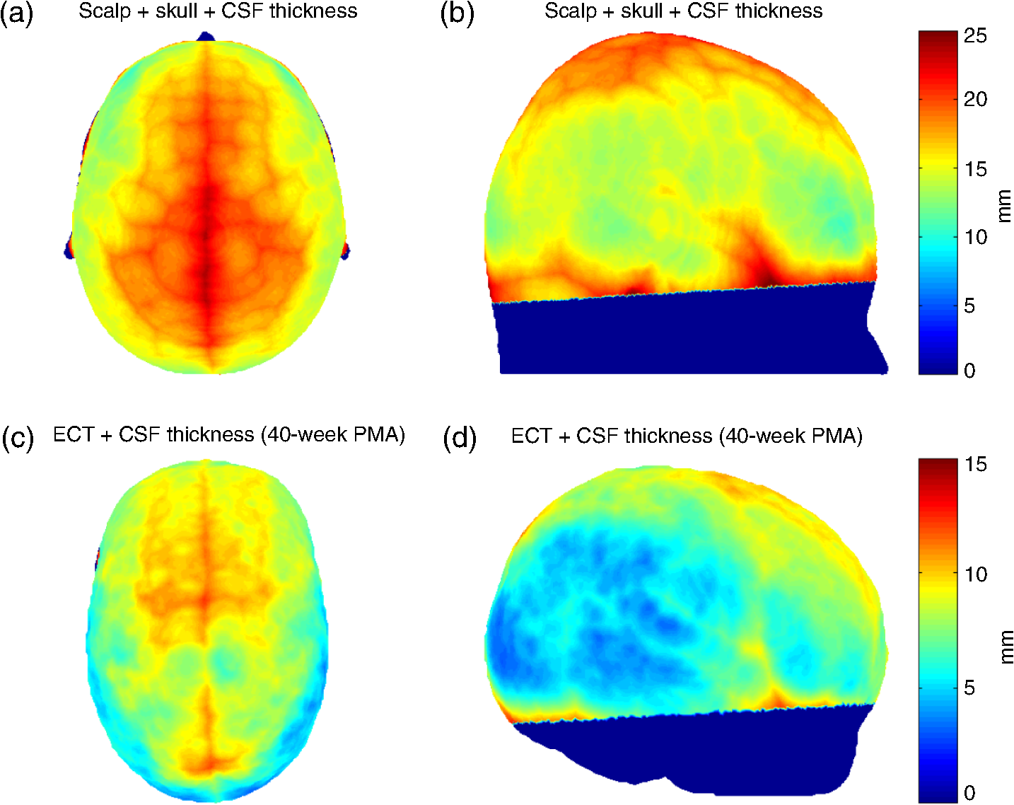 Table 2 contains the median thicknesses of the adult scalp, skull, and CSF tissues for each ROI. Also reported is the most common combination of tissue thicknesses across the whole adult head, as computed using the multivariate histogram approach. Table 2Adult thicknesses (in mm) for scalp, skull, and CSF tissues. Median values for all selected regions of interest (ROIs) and the most common combination of thicknesses for the whole adult head measured as the peak of the multivariate histogram are reported.
Figures 3(a) and 3(b) show the median thickness of the ECT and CSF layers for each age of the 4-D infant head model. Note how the preterm infants tend to exhibit similar values for these thicknesses. In Table 3, the thicknesses of the ECT and CSF tissues are reported for each cluster or age. As expected, both tissue layers are increasing in thickness with increasing age. Fig. 3Median values of (a) the ECT and (b) the CSF thickness for each infant’s age. Younger infants tend to have similar values, which have been grouped into two clusters, cluster 1 from 29- to 33-week PMA and cluster 2 from 34- to 38-week PMA. 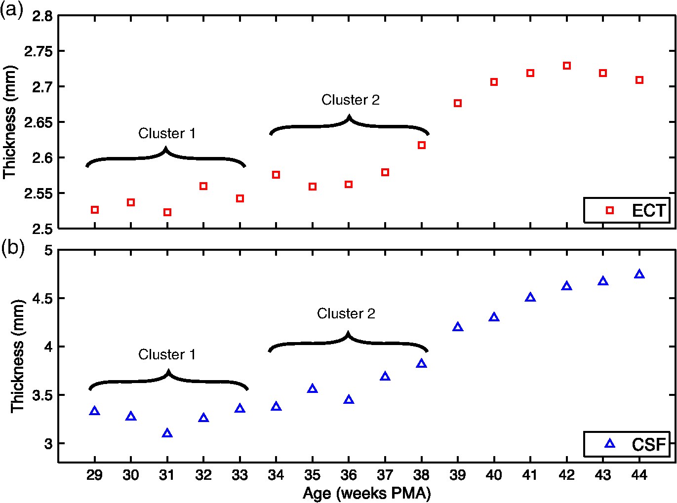 Table 3Infant head model layer thicknesses (in mm) for extra-cerebral tissues (ECT) and CSF tissues. The median value for each cluster or age is reported.
In Fig. 4, the PMDFs at three different source–detector distances in an exemplary model are displayed. Note the relationship between source–detector distance and depth sensitivity. Fig. 4Examples of photon measurement density functions at three different source–detector distances: (a) 30 mm channel, (b) 8 mm channel, and (c) 3 mm channel. The log of the sensitivity is displayed. Only the upper 40 mm of the multilayer slab model is displayed for visualization purposes. The white dashed lines indicate the borders of the tissue layers (between scalp and skull, between skull and CSF, and between CSF and GM, from top to bottom).  Figure 5 shows the values of the POV metric [Figs. 5(a) and 5(d)], the BS metric [Figs. 5(b) and 5(e)], and the RBS metric [Figs. 5(c) and 5(f)] for both adult and infant models across all source–detector separations. The colored area indicates the range of values produced across all models (i.e., all ROIs in the adult and all clusters/ages in the infants) for each source–detector separation. The black line represents the values of the Common model in the adult and the 40-week PMA (term-age) model in the infant. Fig. 5The percentage of overlapping voxels (POV), relative brain sensitivity (RBS), and brain sensitivity (BS) results. (a) and (d) The POV as a function of source–detector separation for adults and infants, respectively. (b) and (e) The BS as a function of source–detector separation for adults and infants, respectively. (c) and (f) The RBS as a function of source–detector separation for adults and infants, respectively. In each case, the red shaded area comprises the range of values exhibited across all models (i.e., across all ROIs in the adult and all clusters/ages in the infant). The black lines are an interpolation of the values obtained in the Common model for the adult and the 40-week PMA model for the infant. Note that Figs. 5(b) and 5(e) include a value for each reference channel (30 mm in adult and 25 mm in infant). 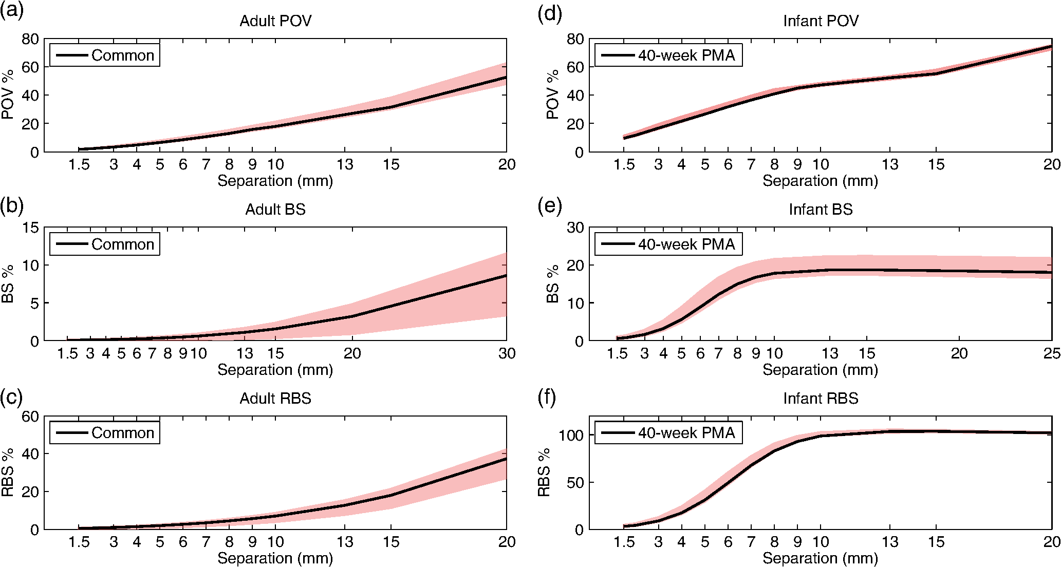 In Fig. 6, the optimum distance for an SS channel is displayed for a given RBS threshold (from 1 to 20%) for each model for both the adult [Fig. 6(a)] and infant [Fig. 6(b)]. Note that a spline interpolation was applied to the computed RBS values to give RBS as a function of short-channel separation in steps of 0.05 mm. The optimum SS channel was then selected as the separation with the highest POV (i.e., the largest separation) that does not exceed the specified RBS threshold. Fig. 6The optimum source–detector distance for a short-separation channel for different RBS thresholds and both (a) adult and (b) infant models. To determine the optimum short-channel separation, first select what RBS threshold is acceptable, and then select the value for most relevant model for your population and probe location. For example, if a 5% RBS value is acceptable and the study in question is of the adult frontal lobe, the optimum short-channel separation would be . 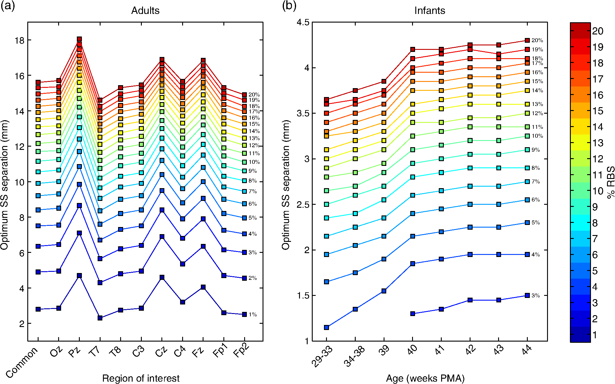 As a further validation of the above results, three additional sets of Monte Carlo simulations were performed. The first was designed to assess the impact of the CSF layer in the infant models. Four additional slab models were produced with a scalp thickness equal to that of the youngest cluster of infants and CSF thicknesses of 0, 1, 2, and 3 mm. The CSF reduced scattering coefficient was also varied between the value used in our simulations () and a higher reduced scattering coefficient () that was previously reported.37 When using the lower value of , the BS as a function of source–detector distance always exhibits a plateau, as was also seen in Fig. 5. The separation at which this plateau occurs increases with decreasing CSF thickness. The BS curve plateaus at for a 1 mm CSF layer. When the higher scattering coefficient is used, BS is still increasing with a separation up to 25 mm, though the trends suggest that a plateau will be reached at greater separations. For a given CSF thickness, the influence of CSF optical properties on BS is very small at short source–detector distances (less than a 3% difference in BS for SS distances ). The second additional set of Monte Carlo simulations was designed to test the impact of the curvature of the head. The BS was calculated for the multiple source–detector distances on the 29-week PMA head model, which should exhibit the highest curvature across our populations. BS as a function of source–detector separation showed similar values and the exact same behavior as that shown in Fig. 5(e), with BS exhibiting a plateau at a source–detector distance of . Last, a set of simulations was performed to assess how significantly the choice of optimum SS distance is affected by the optical properties of tissue. The absorption coefficient of the scalp layer in the Common adult slab model was varied between 0.015 and in steps. This range encompasses all the values of scalp absorption coefficient previously reported.34 The resulting variation in RBS increased as a function of SS distance, with the maximum range found to be 1.6 percentage points for the 20 mm separation. The range of RBS values due to the variation in scalp absorption coefficient for the 8 mm separation was 0.9 percentage points. 4.DiscussionSS channels are essential for accurate fNIRS measurements because they enable the extra-cerebral signal contribution to be regressed from standard separation channels. This reduces the chance that extra-cerebral hemodynamics (which can be temporally correlated with external stimuli) will be falsely interpreted as functional brain activation. Research groups around the world are currently using SS channels with a range of source–detector distance between 5 and 13 mm.12,20,21,24 These different separations will exhibit very different sensitivities to the brain and ECT, which will affect the resulting process of regression and the recovery of functional activation. In this study, we sought to determine how short an SS channel should be to provide a balance between minimizing sensitivity to the brain and maximizing the extra-cerebral sensitivity overlap with a standard separation channel. We performed a series of Monte Carlo simulations on multilayered slab models with tissue thicknesses derived from population-averaged atlases for both adults and newborn infants. While tissue thicknesses vary from person to person, these values are rarely known in advance of an fNIRS study. We have, therefore, created a look-up plot (Fig. 6) that specifies the optimum SS distance in these population-averaged models for a given ROI and an acceptable percentage value of RBS. This percentage value of RBS can be considered to be the average proportion of true functional brain signal that may erroneously be removed in the process of regressing the selected SS channel signal from the standard channel signal. Note, however, that this interpretation assumes a homogenous functional brain activation that is uncorrelated with the superficial signal, and its accuracy will depend on the method of regression. Although this interpretation is limited, at present, the authors do not see a more quantitative method of selecting RBS. In this study, we chose to examine the case where the SS channel is created by the addition of a detector located near to a source that is also used for a standard separation channel. This approach is the most common geometry currently employed because it does not require the use of both a dedicated source and a dedicated detector, and Gagnon et al.13 have shown that employing a dedicated SS channel as close as possible to the standard channel provides the most accurate recovery of functional activity. Note that the results of Fig. 6 would be equally valid in the reciprocal case where an SS channel is formed by placing an additional source close to a detector that is also used for a standard separation channel. This construction is less common because of the risk of detector saturation. For the most common combination of tissue thicknesses in the adult, and a chosen RBS of 5%, the optimum SS in the adult was found to be 8.4 mm. This value is in the expected range given the multiple studies that have demonstrated the benefit of SS channels between 5 and 13 mm.12,20,21,24 To our knowledge, only one study has explicitly tested the impact of changing the SS distance. Goodwin et al.38 reported that a 6 mm separation results in better contrast-to-noise of functional responses than a 13 mm separation and suggested this was due to the non-negligible BS of a 13 mm channel. Our results are consistent with this conclusion. Over the visual cortex, a 13 mm separation will exhibit an RBS of . Our results also show that the choice of optimum SS distance can be very dependent on the location of the array on the adult head. Over the midline (i.e., Cz, Pz, and Fz), a longer SS distance is preferred simply due to the thicker CSF layer that fills the medial longitudinal fissure. However, there is also significant variation away from the midline. The difference between optimum SS distance calculated over the T7 ROI and the C4 ROI differs by as much as 2 mm (Fig. 6). The scalp and skull thicknesses computed in our adult model are in line with literature values.35,39,40 The scalp thickness is higher in the temporal than parieto-occipital and frontal regions, as reported previously.39 The CSF thickness is also in line with previously reported values.35 In the preterm to term infant population, the variability in tissue thicknesses between subjects is extremely high,41 but our calculated scalp to brain distance (i.e., the sum of ECT and CSF thicknesses, Fig. 2) is in line with the limited number of previously reported values.42 Our simulations show that the BS of the reference channel in the adult varies across the scalp between 3.4 and 11.5%, which is also in line with previously reported values.11 The fact that these values are so low further highlights the importance of SS channels as by far the greatest contribution to the measured fNIRS signal comes from the ECT. In line with many previous studies,7,11,35,37 our simulations show that BS in the adult increases with increasing source–detector separation up to 30 mm (Fig. 5). Previous work has shown that this curve will eventually reach a plateau in BS after separation.11,37 One of the most significant challenges to photon transport modeling is the paucity of accurate, tissue-specific optical property values. For the adult models, we selected our absorption and reduced scattering coefficients by fitting all available, published values and selecting the 800 nm wavelength. Because of the need for multilayer models, it was computationally prohibitive to perform a detailed sensitivity analysis to determine and quantify the impact of changing tissue optical properties. However, we did recompute the RBS with a range of scalp absorption coefficients which was judged likely to have the greatest impact on our optimum SS distance computation. These results strongly suggest that Fig. 6 is relatively stable to the choice of optical properties, as RBS was found to vary by, at most, 1.6 percentage points across the range of scalp absorption coefficients. This corresponds to a maximum variation of 0.875 mm in optimum SS distance. This variation is markedly smaller than the variation found between different ROIs. In the infant model, BS also increases with source–detector separation, reaching higher values than in the adult model (Fig. 5), but exhibiting a plateau at a separation of 10 mm. This somewhat surprising result suggests than in the newborn, data from a 10 mm fNIRS channel will contain the same signal contribution from the brain as data from a 20 mm channel. We believe this is due to the impact of the relatively thin ECT layer coupled with a relatively thick CSF layer, a hypothesis that is supported by our additional simulations. The head models that we employed to compute the CSF thickness are the most accurate population-average representation of tissue thicknesses available for the neonatal population, though it is known that the limited contrast of neonatal MRI makes the segmentation of the CSF layer challenging.31 In addition, the values previously reported for the reduced scattering coefficient of CSF in the infant vary considerably, despite the fact that almost all studies cite Ref. 37 as the source of their value. The value we employed was taken from the most recent relevant studies.33,41 Despite this valid concern, our additional simulation results suggest that our calculations of the optimum SS distance in the infant population will not be undermined by uncertainty in the optical properties of the CSF layer. An additional limitation of the work we present here is the use of cuboidal slab geometries instead of head models. We chose this approach for two reasons. First, local variations in anatomy make it difficult to choose a location on a head model that will accurately represent any other location. Second, the use of a slab geometry vastly reduces the number of necessary Monte Carlo simulations. A failure of the slab approach is the absence of curvature. The curvature of the head may be thought to have a significant impact on the BS of a given fNIRS channel, particularly on the infant head where curvature is high. However, we believe that ignoring curvature is a reasonable assumption given that the aim of this study is to examine short separations. Our additional simulations performed in the highest-curvature head model (the 29-week PMA infant) confirmed the suitability of this assumption. In this study, we have used Monte Carlo simulations and the most accurate population-average anatomical models available to produce a look-up plot (Fig. 6) that provides, for an acceptable value of RBS, the optimum SS distance. These values will inform not only current users of fNIRS but also those designing and constructing high-density diffuse optical tomography systems. ReferencesD. A. Boas et al.,
“Noninvasive imaging of cerebral activation with iffuse optical tomography,”
In Vivo Optical Imaging of Brain Function, CRC Press, Boca Raton, Florida
(2009). Google Scholar
F. F. Jöbsis,
“Noninvasive, infrared monitoring of cerebral and myocardial oxygen sufficiency and circulatory parameters,”
Science, 198 1264
–1267
(1977). http://dx.doi.org/10.1126/science.929199 SCIEAS 0036-8075 Google Scholar
S. R. Arridge et al.,
“A finite element approach for modeling photon transport in tissue,”
Med. Phys., 20 299
–309
(1993). http://dx.doi.org/10.1118/1.597069 MPHYA6 0094-2405 Google Scholar
Q. Fang and D. A. Boas,
“Monte Carlo simulation of photon migration in 3D turbid media accelerated by graphics processing units,”
Opt. Express, 17 20178
–20190
(2009). http://dx.doi.org/10.1364/OE.17.020178 OPEXFF 1094-4087 Google Scholar
Q. Fang et al.,
“Accelerating mesh-based Monte Carlo method on modern CPU architectures,”
Biomed. Opt. Express, 3 3223
–3230
(2012). http://dx.doi.org/10.1364/BOE.3.003223 BOEICL 2156-7085 Google Scholar
M. Calderon-Arnulphi, A. Alaraj and K. V. Slavin,
“Near infrared technology in neuroscience: past, present and future,”
Neurol. Res., 31
(6), 605
–614
(2009). Google Scholar
G. E. Strangman, Z. Li and Q. Zhang,
“Depth sensitivity and source-detector separations for near infrared spectroscopy based on the Colin27 brain template,”
PLoS One, 8 e66319
(2013). http://dx.doi.org/10.1371/journal.pone.0066319 1932-6203 Google Scholar
T. Li, H. Gong and Q. Luo,
“Visualization of light propagation in visible Chinese human head for functional near-infrared spectroscopy,”
J. Biomed. Opt., 16 045001
(2011). http://dx.doi.org/10.1117/1.3567085 JBOPFO 1083-3668 Google Scholar
S. Lloyd-Fox, A. Blasi and C. E. Elwell,
“Illuminating the developing brain: the past, present and future of functional near infrared spectroscopy,”
Neurosci. Biobehav. Rev., 34 269
–284
(2010). http://dx.doi.org/10.1016/j.neubiorev.2009.07.008 NBREDE 0149-7634 Google Scholar
G. Taga, F. Homae and H. Watanabe,
“Effects of source-detector distance of near infrared spectroscopy on the measurement of the cortical hemodynamic response in infants,”
Neuroimage, 38 452
–460
(2007). http://dx.doi.org/10.1016/j.neuroimage.2007.07.050 NEIMEF 1053-8119 Google Scholar
G. E. Strangman, Q. Zhang and Z. Li,
“Scalp and skull influence on near infrared photon propagation in the Colin27 brain template,”
Neuroimage, 85
(Pt 1), 136
–149
(2014). http://dx.doi.org/10.1016/j.neuroimage.2013.04.090 NEIMEF 1053-8119 Google Scholar
R. Saager and A. Berger,
“Measurement of layer-like hemodynamic trends in scalp and cortex: implications for physiological baseline suppression in functional near-infrared spectroscopy,”
J. Biomed. Opt., 13 034017
(2008). http://dx.doi.org/10.1117/1.2940587 JBOPFO 1083-3668 Google Scholar
L. Gagnon et al.,
“Short separation channel location impacts the performance of short channel regression in NIRS,”
Neuroimage, 59 2518
–2528
(2012). http://dx.doi.org/10.1016/j.neuroimage.2011.08.095 NEIMEF 1053-8119 Google Scholar
E. Kirilina et al.,
“The physiological origin of task-evoked systemic artefacts in functional near infrared spectroscopy,”
Neuroimage, 61 70
–81
(2012). http://dx.doi.org/10.1016/j.neuroimage.2012.02.074 NEIMEF 1053-8119 Google Scholar
M. Dehaes et al.,
“Quantitative investigation of the effect of the extra-cerebral vasculature in diffuse optical imaging: a simulation study,”
Biomed. Opt. Express, 2 680
–695
(2011). http://dx.doi.org/10.1364/BOE.2.000680 BOEICL 2156-7085 Google Scholar
H. Obrig et al.,
“Spontaneous low frequency oscillations of cerebral hemodynamics and metabolism in human adults,”
Neuroimage, 12 623
–639
(2000). http://dx.doi.org/10.1006/nimg.2000.0657 NEIMEF 1053-8119 Google Scholar
C. Julien,
“The enigma of Mayer waves: facts and models,”
Cardiovasc. Res., 70 12
–21
(2006). http://dx.doi.org/10.1016/j.cardiores.2005.11.008 CVREAU 0008-6363 Google Scholar
R. B. Saager and A. J. Berger,
“Direct characterization and removal of interfering absorption trends in two-layer turbid media,”
J. Opt. Soc. Am. A, 22 1874
(2005). http://dx.doi.org/10.1364/JOSAA.22.001874 JOAOD6 0740-3232 Google Scholar
L. Gagnon et al.,
“Further improvement in reducing superficial contamination in NIRS using double short separation measurements,”
Neuroimage, 85
(Pt 1), 127
–135
(2014). http://dx.doi.org/10.1016/j.neuroimage.2013.01.073 NEIMEF 1053-8119 Google Scholar
L. Gagnon et al.,
“Improved recovery of the hemodynamic response in diffuse optical imaging using short optode separations and state-space modeling,”
Neuroimage, 56 1362
–1371
(2011). http://dx.doi.org/10.1016/j.neuroimage.2011.03.001 NEIMEF 1053-8119 Google Scholar
F. Scarpa et al.,
“A reference-channel based methodology to improve estimation of event-related hemodynamic response from fNIRS measurements,”
Neuroimage, 72 106
–119
(2013). http://dx.doi.org/10.1016/j.neuroimage.2013.01.021 NEIMEF 1053-8119 Google Scholar
Q. Zhang, G. E. Strangman and G. Ganis,
“Adaptive filtering to reduce global interference in non-invasive NIRS measures of brain activation: how well and when does it work?,”
Neuroimage, 45 788
–794
(2009). http://dx.doi.org/10.1016/j.neuroimage.2008.12.048 NEIMEF 1053-8119 Google Scholar
S. Wang et al.,
“Effects of spatial variation of skull and cerebrospinal fluid layers on optical mapping of brain activities,”
Opt. Rev., 17 410
–420
(2010). http://dx.doi.org/10.1007/s10043-010-0076-6 1340-6000 Google Scholar
N. M. Gregg et al.,
“Brain specificity of diffuse optical imaging: improvements from superficial signal regression and tomography,”
Front. Neuroenergetics, 2 14
(2010). http://dx.doi.org/10.3389/fnene.2010.00014 FNREJG 1662-6427 Google Scholar
V. Fonov et al.,
“Unbiased average age-appropriate atlases for pediatric studies,”
Neuroimage, 54 313
–327
(2011). http://dx.doi.org/10.1016/j.neuroimage.2010.07.033 NEIMEF 1053-8119 Google Scholar
K. L. Perdue and S. G. Diamond,
“T1 magnetic resonance imaging head segmentation for diffuse optical tomography and electroencephalography,”
J. Biomed. Opt., 19 026011
(2014). http://dx.doi.org/10.1117/1.JBO.19.2.026011 JBOPFO 1083-3668 Google Scholar
Q. Fang and D. A. Boas,
“Tetrahedral mesh generation from volumetric binary and grayscale images,”
in 2009 IEEE Int. Symp. on Biomedical Imaging: From Nano to Macro,
1142
–1145
(2009). Google Scholar
R. Bade, J. Haase and B. Preim,
“Comparison of fundamental mesh smoothing algorithms for medical surface models,”
in Proc. Simul. Vis.,
289
–304
(2006). Google Scholar
S. Brigadoi et al.,
“A 4D neonatal head model for diffuse optical imaging of pre-term to term infants,”
Neuroimage, 100 385
–394
(2014). http://dx.doi.org/10.1016/j.neuroimage.2014.06.028 NEIMEF 1053-8119 Google Scholar
M. Dehaes et al.,
“Quantitative effect of the neonatal fontanel on synthetic near infrared spectroscopy measurements,”
Hum. Brain Mapp., 34 878
–889
(2013). http://dx.doi.org/10.1002/hbm.v34.4 HBRME7 1065-9471 Google Scholar
G. Strangman, M. A. Franceschini and D. A. Boas,
“Factors affecting the accuracy of near-infrared spectroscopy concentration calculations for focal changes in oxygenation parameters,”
Neuroimage, 18 865
–879
(2003). http://dx.doi.org/10.1016/S1053-8119(03)00021-1 NEIMEF 1053-8119 Google Scholar
A. Custo et al.,
“Effective scattering coefficient of the cerebral spinal fluid in adult head models for diffuse optical imaging,”
Appl. Opt., 45 4747
–4755
(2006). http://dx.doi.org/10.1364/AO.45.004747 APOPAI 0003-6935 Google Scholar
F. Bevilacqua et al.,
“In vivo local determination of tissue optical properties: applications to human brain,”
Appl. Opt., 38 4939
–4950
(1999). http://dx.doi.org/10.1364/AO.38.004939 APOPAI 0003-6935 Google Scholar
Y. Fukui, Y. Ajichi and E. Okada,
“Monte Carlo prediction of near-infrared light propagation in realistic adult and neonatal head models,”
Appl. Opt., 42 2881
–2887
(2003). http://dx.doi.org/10.1364/AO.42.002881 APOPAI 0003-6935 Google Scholar
J. R. Goodwin, C. R. Gaudet and A. J. Berger,
“Short-channel functional near-infrared spectroscopy regressions improve when source-detector separation is reduced,”
Neurophotonics, 1 015002
(2014). http://dx.doi.org/10.1117/1.NPh.1.1.015002 NEUROW 2329-423X Google Scholar
F. Babiloni et al.,
“A high resolution EEG method based on the correction of the surface Laplacian estimate for the subject’s variable scalp thickness,”
Electroencephalogr. Clin. Neurophysiol., 103 486
–492
(1997). http://dx.doi.org/10.1016/S0013-4694(97)00035-7 ECNEAZ 0013-4694 Google Scholar
W. H. Oldendorf and Y. Iisaka,
“Interference of scalp and skull with external measurements of brain isotope content. 1. Isotope content of scalp and skull,”
J. Nucl. Med., 10 177
–183
(1969). JNMEAQ 0161-5505 Google Scholar
J. Heiskala et al.,
“Probabilistic atlas can improve reconstruction from optical imaging of the neonatal brain,”
Opt. Express, 17 14977
–14992
(2009). http://dx.doi.org/10.1364/OE.17.014977 OPEXFF 1094-4087 Google Scholar
M. S. Beauchamp et al.,
“The developmental trajectory of brain-scalp distance from birth through childhood: implications for functional neuroimaging,”
PLoS One, 6 e24981
(2011). http://dx.doi.org/10.1371/journal.pone.0024981 1932-6203 Google Scholar
BiographySabrina Brigadoi received her PhD degree from Padova University, Italy. Currently, she is a research associate in the Biomedical Optics Research Laboratory, University College London, United Kingdom. Her research interests are focused on signal processing techniques for functional near-infrared spectroscopy and head model development for optical imaging techniques. In particular, she is interested in motion artifact correction and physiological noise reduction techniques and in creating a developmental accurate head model for optical imaging reconstruction. Robert J. Cooper studied physics at New College Oxford before receiving a PhD degree in medical physics from University College London. His research has focused on advancing fNIRS and diffuse optical imaging techniques, with emphasis on clinical applications including epilepsy and neonatal brain injury. Formerly, he was a research fellow at the Martinos Center for Biomedical Imaging, Harvard Medical School. He has since returned to University College London in order to develop a specialized neonatal functional imaging group. |
|||||||||||||||||||||||||||||||||||||||||||||||||||||||||||||||||||||||||||||||||||||||||||||||||||||||||||||||||||||


