|
|
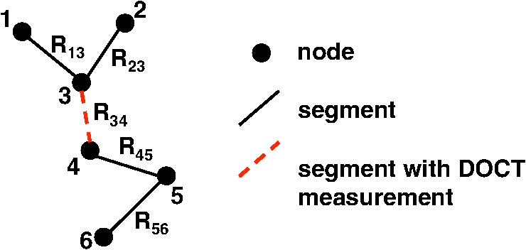
1.IntroductionThere is increasing interest in modeling microvascular cerebral blood flow () to better guide our understanding of neuroimaging methods1,2 and cerebrovascular physiology.3 Several groups have performed the computation of in realistic vascular networks.4–14 Several difficulties arise when the computation takes place over a real vascular network measured in vivo. This includes vessel diameter estimation and, therefore, estimation of resistances. Moreover, the truncation of the network at the edges of the imaging volume inevitably increases the number of boundary conditions required for the computation of .7,12 All of these issues increase the uncertainty of the microvascular flow distributions computed with these models and limit their application. Doppler optical coherence tomography (DOCT) applied to the cerebral microvasculature has recently been demonstrated15 and validated16 to evaluate flow in a small number of vessels. Such measurements could, in principle, guide and improve the estimation of in truncated microvascular networks. Using simulations, we investigate the error reduction obtained by using DOCT measurements to constrain the estimation of microvascular flow distributions along the vascular network. We then apply our method to in vivo data by combining DOCT for quantitative measurement of microvascular blood flow in specific vessels and two-photon laser scanning microscopy (TPLSM) for precise measurement of the three-dimensional (3-D) vessel architecture. 2.TheoryWe represent a vessel network as a graph consisting of nodes joined by segments as illustrated in Fig. 1. The flow in a given segment of length and diameter is computed according to Poiseuille’s law where the term is the resistance to flow of the segment and is the pressure gradient between the two nodes of the segment. is the viscosity of blood and was set to in our work.17,18 More complex models described in the literature7,17,19 could be used similarly. Note that this is true as long as the hematocrit is assumed to be constant across the vascular network; otherwise, an iterative approach has to be used.4 Conservation of flow at branching nodes implies that where denotes the flow from to .If we first ignore the DOCT measurement in segment 3-4, we substitute Eq. (1) into Eqs. (2) to (4) to get In addition to flow conservation, boundary conditions for blood pressure need to be established at the graph end points. In this work, these values were taken from the literature18 based on the diameter of the vessel. For the simple graph of Fig. 1, one gets Equations (5) to (10) can be written in matrix form where is a 6-by-6 matrix, is a vector containing the pressure of all nodes, and is a vector containing the right-hand side of Eqs. (5) to (10). The pressure for all nodes can be solved simultaneously by inverting Eq. (11).Two different approaches can be used to take into account the DOCT measurement in segment 3-4 (labeled ). The first method is to add a seventh equation to the linear system of Eq. (11): In this case, the system become overdetermined and must be solved with a least square fitting procedure such as lsqlin in Matlab. Overconstraining the system with the addition of DOCT measurements helps to alleviate the impact of estimated vessel resistances and the assumption about pressure boundary conditions. The second method uses the DOCT measurement as a hard constraint (i.e., assuming that this value represents the true flow) and to construct the following solvable linear system: which together with Eqs. (8) to (10) can be written in matrix form where the subscript stands for constrained. In this case, neither the diameter nor the length of the segments containing a DOCT measurement is taken into account in the computation of flow.Both methods were tested and the first method (overdetermined system) resulted in minor improvements compared to the second method (hard constraint). While the overdetermined method considers the resistance value of the vessels containing a DOCT measurement in the least square procedure, the hard constraint method totally avoids this resistance value. Since most of the error comes from the computation of the resistance of the vessels from their diameter, this results in a better improvement for the hard constraint method compared to the overdetermined method. We, therefore, chose the hard constraint method for all the results presented in this work. 3.Material and Methods3.1.Numerical SimulationsWe investigated the improvement obtained by adding DOCT measurements to the recovery procedure using a synthetic vessel network. The synthetic network contained 175 nodes and 240 vessel segments, including 1 inflowing arteriole and 3 outflowing venules, as shown in Fig. 2(a). The capillary nodes connected three capillaries, which is the typical configuration measured experimentally.20 The diameter of the arteriole and the venules was set to , whereas the diameter of the capillaries was fixed to . The length of all vessels was set to . Pressure boundary condition was set to 105 mmHg in the inflowing arteriole and to 10 mmHg in the outflowing venules. The pressure at the end node capillaries was set between 30 and 80 mmHg depending on the position in the network. Flow was first computed given this set of boundary conditions. The noise was then introduced by randomly varying the values for the pressure boundary conditions and the resistance of the vessels. Noise level was set to 25% (max/mean) for pressure boundary conditions which is of the order of the variability measured experimentally.18 Noise in the arterial and venous resistance was set to 25%, which corresponds to an experimental error in the diameter estimation of 5% to 6% (15 to ). For the capillary resistances, the error in the experimental diameter estimation is also but since the mean diameter of capillaries is about , this corresponds to an error of 20% which transforms into an error of 100% in the resistance calculation. We, therefore, used 100% for the noise of the capillary resistance in our simulations. Flow was then recovered using the erroneous pressure boundary conditions and resistance values without DOCT priors using Eq. (11). A fraction of the vessels were then randomly selected and DOCT priors were set for these vessels. Flow was then reconstructed using these priors from Eq. (16). The fraction of vessels with DOCT priors ranged from 2 to 10%. The value for the DOCT measurements was set to the true (simulated) flow value with noise added. Different levels of noise for the DOCT values were tested ranging from 5% to 25%. The performance was quantified by computing the mean squared error (MSE) between the simulated and the recovered flow in both cases (i.e., with and without DOCT priors). To insure reproducible results, the simulations were run 500 times with different noise instances for boundary conditions and resistance values. MSE values were averaged across all 500 simulations. Fig. 2Simulations showing the improvement in accuracy obtained by integrating DOCT measurements in the computation of flow. The fraction of vessels with DOCT was 10% and noise in the DOCT measurement was 10%. (a) Segments containing DOCT priors. (b) Error map in percent for flow recovered with and without priors. (c) Comparison of the MSE obtained for different configurations simulated. Each bar represents the average MSE obtained for 500 simulations with different DOCT prior configurations and different noise instances. Simulations were run with 10% DOCT priors located only in the capillaries, with 10% DOCT priors located anywhere but including one, two and three outflowing venules, and with 10% DOCT priors located anywhere but including the inflowing arteriole. 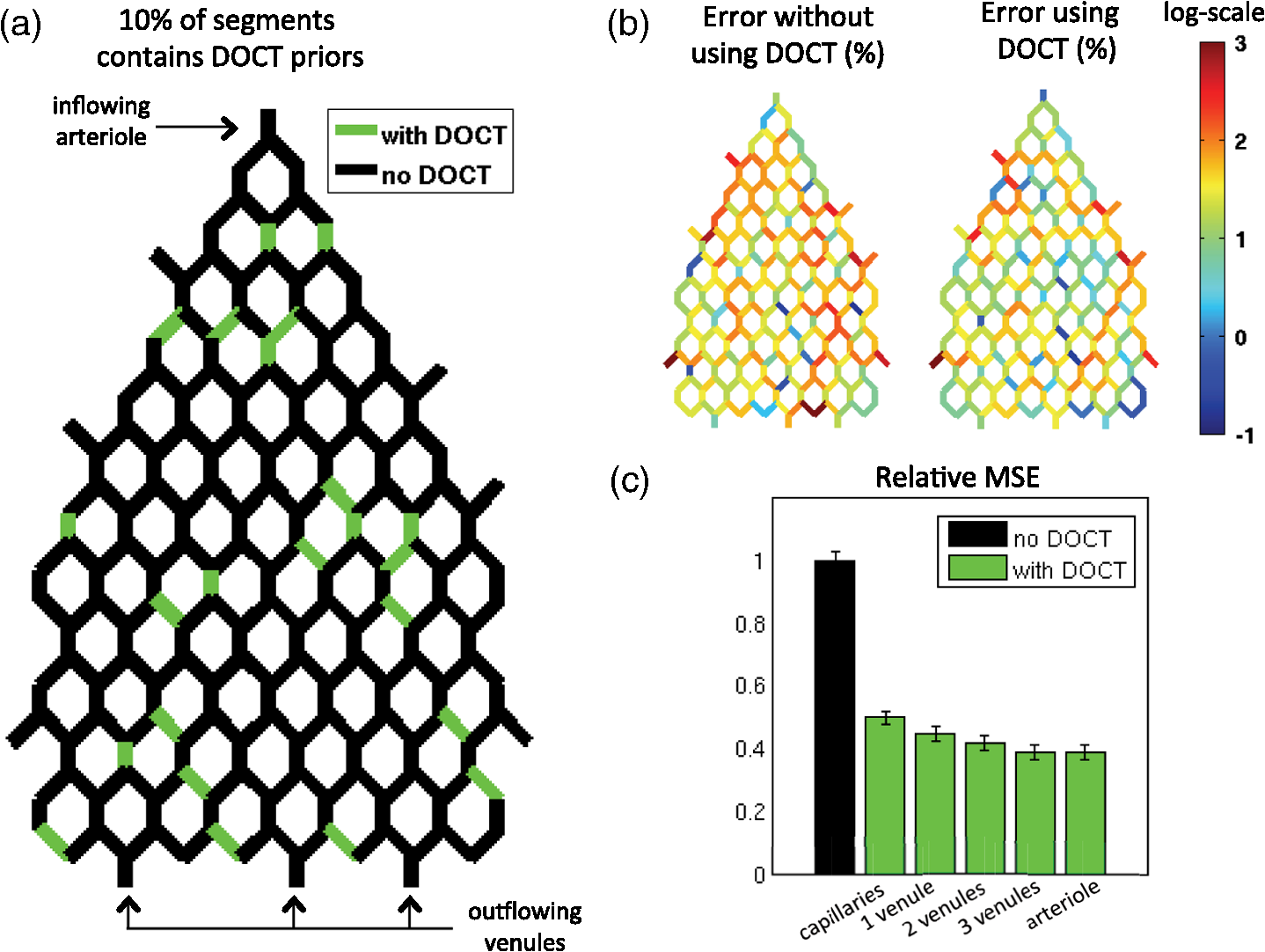 3.2.Animal PreparationAnimal protocols were approved by the Massachusetts General Hospital Subcommittee on Research Animal Care. We anesthetized a C57BL/6 mouse (male, 25 g) with isoflurane (1-2% in a mixture of and air) under constant temperature (37°C). We then opened a 2.5-mm-wide cranial window over the primary somatosensory cortex with the center of the window in the parietal bone 2 mm posterior from the bregma and 2 mm lateral from midline, removed the dura, and sealed the window with a microscope coverslip. We used a catheter in the femoral artery to administer the dyes, to continuously monitor the blood pressure and heart rate, and to sample systemic blood gases ( and ) and pH. During the measurement period, the isoflurane anesthesia was reduced to 0.7% to 1.2% and the following physiological parameters were maintained: arterial , arterial , and mean arterial . 3.3.Multimodal MicroscopeOur multimodal microscope, described in Sakadžić et al.,21 has independent TPLSM and OCT scanning arms that share the same imaging objective. This allows for easy switching between sequential TPLSM and OCT measurements. The TPLSM optical beam was scanned in the plane by galvanometer scanners (6215H, Cambridge Technology, Inc.). An electro-optic modulator (ConOptics, Inc.; extinction ratio 500) served to gate the output of a Ti:Sapphire oscillator (840 nm, 80 MHz, 110 fs, Mai-Tai, Spectra-Physics). The pulse duration was 350 fs (assuming a pulse shape), as measured at the sample. The emission was reflected by a dichroic mirror (LP 735 nm, Semrock) and detected with a large collection efficiency () by a detector array, consisting of four independent photomultiplier tubes. DOCT is a path length-resolving optical imaging technique that can measure velocity axial projections in well-defined microscopic volumes. These axial projections can be used to perform absolute measurements of blood flow. DOCT has been applied to brain microvasculature15 and validated against hydrogen clearance methods.16 DOCT can achieve a spatial resolution of in the transverse plane and 3 to in the axial direction. The penetration in cortical tissue can reach beyond 1 mm. The temporal resolution for CBF measurement in a single vessel is on the order of 0.1 s and the time required to image an entire volume of is . A superluminescent diode (model EX8705-2411, Exalos Inc.) with a center wavelength of 856 nm, bandwidth of 54 nm, and a power of 5 mW was used as the light source. The axial (depth) resolution was in air ( in tissue) after spectral shaping. The power on the sample was 1.5 mW, enabling a maximum sensitivity of 99 dB. A home-built spectrometer using a 2048 pixel, 12-bit line scan camera (Aviiva SM2 camera, e2v Semiconductors) enabled an imaging speed of 22,000 axial scans per second and an axial imaging range of 2.5 mm in air. The transverse resolution was . Two pairs of galvanometer mirrors (Cambridge Technology, Inc.) were used to independently scan the TPLSM and OCT beams. The galvanometer mirrors were relay imaged onto the back focal plane of a microscope objective (Olympus XLUMPLFL20XW/IR, 0.95 NA, water immersion, 2 mm working distance). The TPLSM and OCT optical beams were coupled into the microscope objective by a movable dichroic mirror. A motorized stage controlled the focal position by moving the objective along the vertical axis (). Both TPLSM and OCT systems were controlled by custom-designed software written in LabView (National Instruments). 3.4.Experimental MeasurementsWe first performed a DOCT scan protocol for quantitative flow measurements. The details of the scanning protocol can be found in Srinivasan et al.15 The DOCT scan generated a 3-D map of the axial () projection of velocity. The resolution of our OCT was 10 to , preventing velocity estimates in capillaries because of partial volume effects. In addition, the system could only measure velocity projections in the range which can potentially create phase wrapping in large arteries. Because of these two limitations, DOCT measurements were only considered in larger ascending venules in this work. When the resolution of the DOCT scan is smaller than the diameter of the vessels, the flow at specific locations in a vessel is obtained by summing the velocity axial projection over the vessel area in the en face (also known as transverse or ) plane.15 In this work, an alternative method was used to avoid partial volume effects. The flow in a given vessel was computed from the maximal velocity measured in this vessel and the diameter of the vessel measured from the TPLSM angiogram, assuming a parabolic flow profile. The maximal velocity was obtained from the DOCT velocity axial projection by correcting for the angle between the longitudinal direction of the vessel and the axial direction of the OCT beam. Since ascending venules are almost parallel to the OCT beam, these angular corrections were very small. Blood plasma was then labeled with fluorescein isothiocyanate-conjugated dextran (FITC) at 500 nM concentration in blood. We then acquired a stack of the FITC-labeled vasculature using TPLSM ( voxel size) as described in Sakadžić et al.21 Although OCT can also be used to generate angiograms, the spatial resolution and contrast-to-noise ratio is generally higher with FITC TPLSM, which makes it easier to graph (i.e., vectorize) the vascular stack in the subsequent steps. This data was previously published in Sakadžić et al.21 and Gagnon et al.22 3.5.Data ProcessingThe TPLSM angiogram was graphed with a custom software using a combination of automatic segmentation procedures and manual corrections.5,23 Vessel diameter was estimated at each graph node by thresholding the image at a low value of of the maximum image intensity, considering lines through the node point oriented every 3 deg in the local plane perpendicular to the vessel axis, and finding the minimum distance from vessel edge to vessel edge. To reconstruct flow in the experimental vessel network, we set the blood pressure boundary condition for the arterioles and venules crossing the sides of the imaged volume using tabulated values from Ref. 18 given the vessel diameter and the vessel type (arteriole or venule). Similarly to our simulations, pressure boundary condition was set to 105 mmHg in the inflowing arteriole and to 10 mmHg in the outflowing venules. This set of boundary conditions has been shown to result in accurate and realistic flow distributions in previous studies.5,12 4.Results and Discussion4.1.Simulations ResultsThe results of our simulations are shown in Fig. 2. In the case of this specific output, 10% of the vessel segments contained DOCT priors. A random noise was added to each of those DOCT priors and the maximum amplitude of the noise was set to 10% of the flow value for each segment. Figure 2(a) shows the specific segments that contained a DOCT prior for this specific simulation. Figure 2(b) shows the error map in percent with and withtout DOCT priors. We first observe that the residual error in both cases is not located around particular vessels. It is rather spread across the entire network. We also observe a reduction in the error of the reconstructed flow using DOCT priors. The error reduction is spread across the network and is not limited around vessels containing a DOCT prior or restricted to inflowing or outflowing vessels. To account for the variability introduced by the noise, simulations were run 500 times with different noise instances and different configurations for the DOCT priors. The average residual error in the reconstructed flow was 300% without DOCT measurements and 150% when 10% of the segments contained DOCT measurements, even if those measurements contained 25% noise. The high level of residual error in the reconstructed flow is the result of a high noise in the resistance of the capillaries which was set to 100%. Figure 2(c) shows the comparison of the MSE between the simulated and the recovered with and without the DOCT priors. Each bar represents the average MSE obtained from 500 simulations with different noise instances and different DOCT prior configurations. Simulations were run with 10% DOCT priors located only in the capillaries, with 10% DOCT priors located in any vessels including 1, 2 and 3 outflowing venules, respectively, and with 10% DOCT priors located in any vessels including the inflowing arteriole. Note that vessels with DOCT priors did not contribute to the MSE calculation and thus did not bias the results. We observe that constraining the flow reconstruction with DOCT priors in 10% of the vessels reduced the MSE to 50% of the MSE obtained when no DOCT priors were used. When the vessels with priors included 1, 2 and 3 outflowing venules, the MSE was further reduced to 45, 42, and 39% of the MSE obtained with no DOCT prior, respectively. The same reduction to 39% of the initial MSE was obtained when the vessels with priors included the inflowing arteriole. Constraining the flow value in the inflowing arteriole or an outflowing venule will null the impact of the pressure boundary condition for this specific vessel and several downstream vessels (or upstream vessels for the case of a venule) since flow must be conserved along the vascular tree. We note that constraining the flow in a single outflowing venule still reduces the MSE compared to the case where the DOCT priors were located only in the capillaries. Moreover, constraining the flow in the inflowing arteriole or all the outflowing venules will fix the regional blood flow (or the global perfusion) of the network and results in global lower MSE. These results indicate that getting DOCT measurements in large inflowing arterioles or large outflowing venules will have the most impact on the flow computation. Simulations were run with different noise levels and different fractions of segments containing DOCT priors. Averaged results are presented in Fig. 3. Each data point corresponds to an average over 500 simulations. Panel (a) corresponds to simulations where the vessels with DOCT priors were located in the capillaries only, whereas panel (b) corresponds to simulations where the vessels with DOCT priors included either the inflowing arteriole or all three outflowing venules. Note that the top line corresponds to DOCT priors only in the inflowing artery or in all the outflowing veins (no priors in capillaries). Greater reduction in MSE was obtained by increasing the number of vessel segments with DOCT priors compared with reducing the DOCT noise. We also note that the difference obtained by including the inflowing arteriole or the outflowing venules is more meaningful if the number of DOCT priors is lower. Specifically, the improvement doubled when 2% of the segments contained DOCT priors (from 12% to 24%) compared to a less meaningful difference (from 50% to 60%) when 10% of the segments contained DOCT measurements. Fig. 3Averaged results of the simulations. The improvement in MSE with DOCT priors is shown for different levels of noise and different fraction of segments containing DOCT priors. (a) Vessels with DOCT priors were located only the capillaries. (b) Vessels with DOCT priors included the inflowing arteriole or all three outflowing venules. 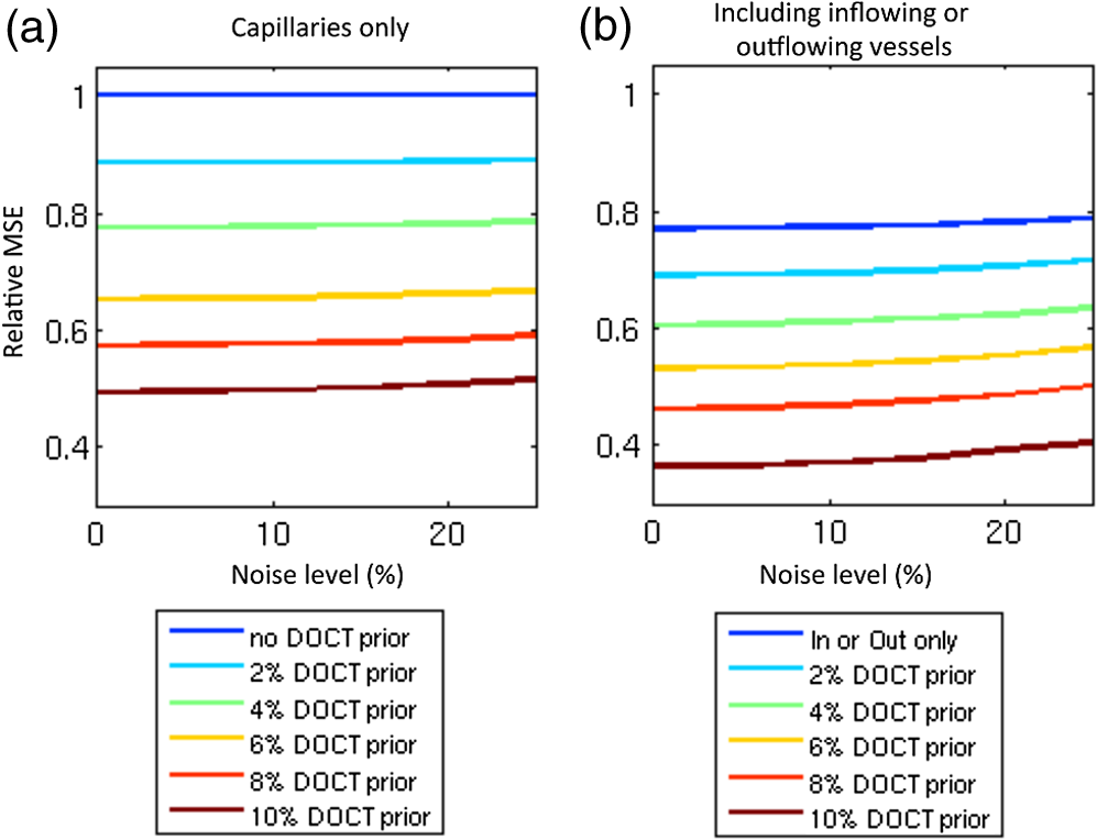 4.2.Reconstruction of μCBF from Experimental Measurements on a MouseThe FITC-labeled vasculature measured with TPLSM is shown in Fig. 4(a) where a maximum intensity projection is displayed over the first of the mouse cortex. This vascular stack and the DOCT measurements were previously published in Sakadžić et al.21 and Gagnon et al.22 A high contrast-to-noise ratio can be appreciated and this feature allowed the vascular network to be graphed (see Sec. 3). A slice of the corresponding DOCT velocity projection volume is shown in Fig. 4(b). Segments colored in blue correspond to blood flowing down into the brain (usually penetrating arterioles) while segments colored in red correspond to blood flowing out of the brain (generally ascending venules), although in this example we do see undulations of large surface vessels. Nine outflowing venous segments contained DOCT flow measurements. From our simulation results [the top line of Fig. 3(b)], we estimate the MSE in the reconstructed blood flow to be 80% of the MSE that we would have obtained without DOCT measurements. This corresponds to an improvement of 20%. Fig. 4Reconstruction of flow in the mouse cortex. (a) Two-photon microscopy FITC angiogram. (b) Doppler OCT velocity image. (c) reconstructed from the model with constraints from the DOCT measurements. 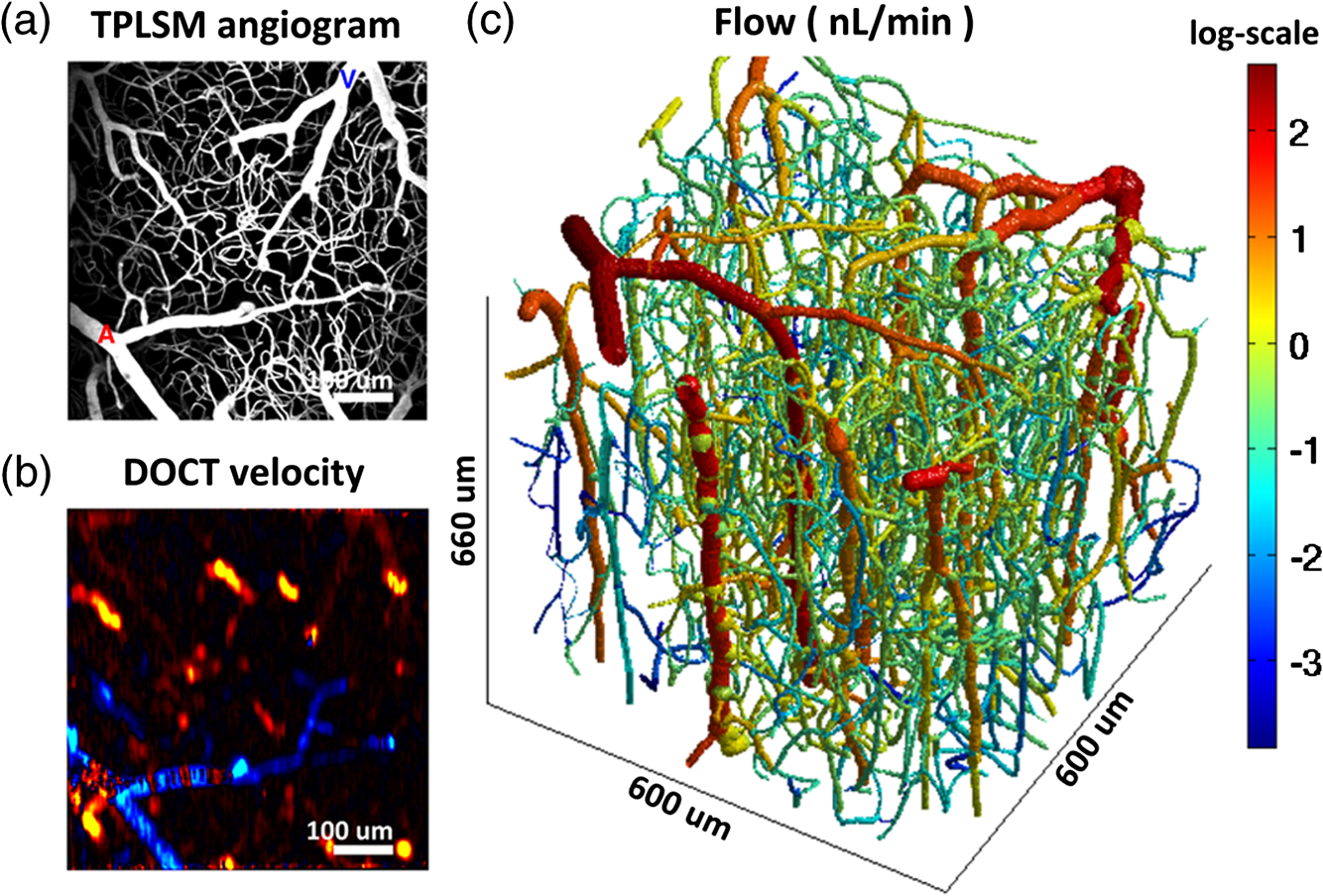 The resulting distribution reconstructed from the multimodal approach (i.e., using the DOCT constraints in ascending venules) is shown in Fig. 4(c). Values of 15 to were reconstructed for the absolute in the ascending venules which is in agreement with values previously reported for rats anesthesized with isofluorane (20 to and 25 to ).15,16 The reconstructed was larger in penetrating arterioles compared to ascending venules since the number of penetrating arterioles was lower than the number of ascending venules—a feature of the mouse cortical microvasculature previously reported in the literature.20 We note that the reconstructed in the capillary bed was very heterogeneous, which is consistent with recent measurements of capillary flux across the rat cortex.24 Our multimodal approach enables us to estimate blood pressure at every branching point of the vascular network and blood velocity in all segments. The reconstructed blood pressure drop from arterioles to venules is shown in Fig. 5(a) while the velocity profile is plotted in Fig. 5(b). The values reconstructed are superimposed with experimental values of blood pressure measured on cats18 and blood velocity measured on mice.25 As shown in Fig. 5, a good agreement was obtained between the reconstructed values and the values previously reported. Our velocities for capillaries are also in good agreement with values reported in the rat cortex (between 0.5 and ).25–28 Sources of error for capillary velocities include the estimation of the diameter of the capillaries. The mean diameter of the capillaries was in our experimental vascular network. Fig. 5(a) Blood pressure and (b) blood velocity reconstructed in the mouse cortex from the multimodal data set as a function of vessel type and diameter. Error bars represent standard error on the mean. Values from Lipowsky18 and Santisakultarm et al.25 are also displayed for comparison. 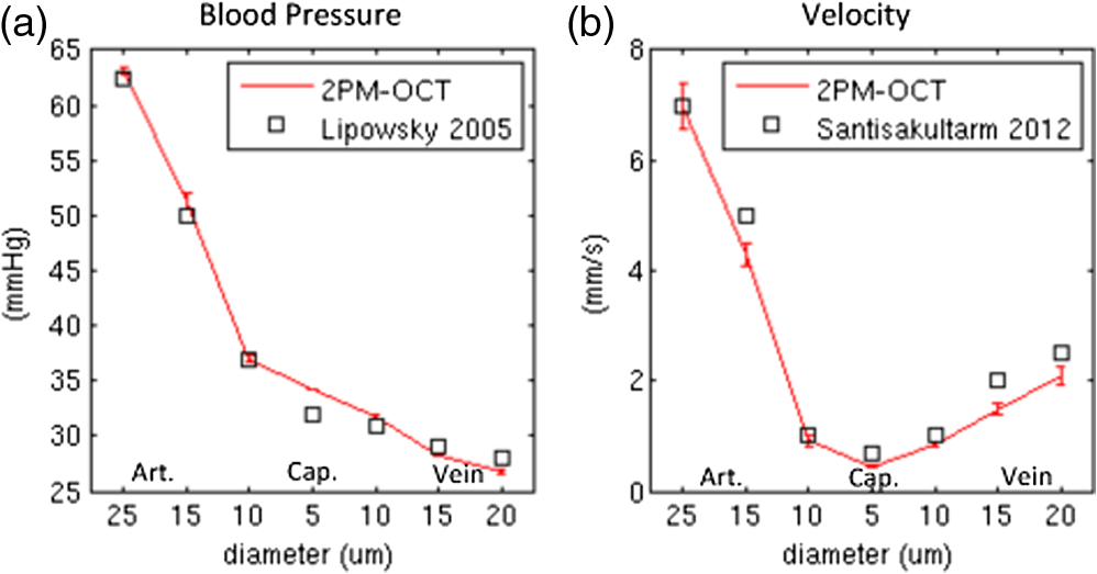 The reconstructed blood pressure dropped sharply from the arteriole to the first branches of the precapillary arterioles indicating that arterioles are a major source of resistance in this microvascular network. The velocity profile decreased from the arterioles to the capillary bed and increased from the capillaries to the venules. This feature is explained by the fact that the total cross-section of the vasculature is larger in the capillary bed compared to arterioles and venules. This behavior was also obtained in previous works simulating blood flow in two-dimensional synthetic vascular networks.6 The velocity in the venules stayed lower compared to the arterioles because of the higher cross-sectional area of venules compared to arterioles in a mouse. 4.3.Calculation of Regional Blood FlowThe reconstructed presented here in Fig. 4 can be used to calculate regional blood flow of the entire vascular stack. This can be achieved by summing either the flow of all inflowing vessels or the flow of all outflowing vessels and assuming or measuring the cortical thickness. This can be viewed as a forward or direct problem and is very straightforward to perform. Assuming a cortical thickness of 1.2 mm,29 the result for the stack of Fig. 4 was which is good agreement with values reported in the literature.30 Back-calculating given a regional blood flow measurement represents the corresponding inverse problem and is more difficult to perform. One thing to note is that back-calculating flow in individual inflowing or outflowing vessels given a regional blood flow measurement does not require the entire reconstruction of as presented in this work. In the case where a single inflowing arteriole feeds the vascular stack, one can directly compute the flow in the single inflowing arteriole from its diameter (assuming or given a measurement of the cortical thickness). The same thing happens if a single outflowing venule drains the entire stack. However, as the number of inflowing arteries or outflowing venules become , there exist multiple solutions to the inverse problem. In this case, flow measurements in individual inflowing or outflowing vessels are needed as well as diameter measurements in the remaining inflowing or outflowing vessel. 4.4.Potential ApplicationsThe change in CBF during healthy aging is an active area of research.27,31 The numerical method presented in this work has phe otential to investigate age-related differences in CBF at the microvascular level based on measurements of relevant CBF parameters.27 Specifically, our method will allow us to reconstruct with better accuracy in the aged rodent cortex which might reveal differences in microvascular circulation between young and aged mice. This will potentially allow us to make predictions about macroscopic flow parameters that can be measured noninvasively in humans studies. Although our multimodal reconstruction method reduces the error on flow reconstruction by 50%, our simulations indicate that the residual error is still on the order of 150%. Most of this error comes from the capillary bed and is dominated by uncertainty in capillary diameter estimation. This high level of noise in the reconstructed limits the application of our method to study phenomena that only modify capillary blood flow distribution.3 However, the residual error in the regional blood flow is lower and is of the order of the noise in the experimental DOCT measurements in the inflowing or outflowing vessels. Our method can, therefore, be used to study phenomena which modify regional blood flow such as aging.27,31 4.5.Limitations and Future StudiesAs mentioned before, the resolution of our OCT system was 10 to , which did not permit measurement of flow in the capillary bed. New methods were recently developed24,32–34 to measure in the capillary network. These measurements could be included in our computational framework in future studies. Another limitation of our system is the low readout rate of our OCT camera limiting the measured velocity projections to . This can potentially create phase wrapping in large arterioles, therefore, we limited our DOCT measurements to venules. A faster OCT system like the one used in Srinivasan et al.16 could resolve this issue and allow us to constrain flow reconstruction in both arterioles and venules. It is worth mentioning that the simulations performed in the first part of this work did not assume any specific modality for the measurement of CBF in individual vessels. Rather, the simulations focused on the improvement that can potentially be obtained by constraining the flow reconstruction with any experimental flow measurement. In our case, we chose to use DOCT for the flow measurements since our multimodal microscope allowed for such experiments. Nevertheless, one could have chosen to perform the flow measurement with TPLSM line scan measurements26 instead. We will mention here that DOCT has some advantages over TPLSM such as faster acquisitions.15 New experimental methods permit capillary flow speed measurements on several vessels simultaneously.24,34,35 These methods will allow us to validate our computational method in future studies and potentially improve it by providing more measurements that can be used to constrain the flow reconstruction. Moreover, these measurements will allow us to measure temporal variation in while our computational method assumes a steady-state flow. 5.ConclusionIn conclusion, we presented a computational framework to compute across real microvascular angiograms with the help of Doppler OCT flow measurements as priors. We demonstrated that adding flow constraints results in more accurate reconstruction of microvascular blood flow in incomplete or truncated microvascular networks. Moreover, the localization of these measurements is important and more improvements are obtained if the flow measurements are located around inflowing arterioles or outflowing venules. Our simulations showed that measuring flow in 10% of the vessels can reduce the error by 50%. We finally applied our computational framework to a multimodal data set collected over the mouse cortex. Our data contained two-photon microscopy angiography together with quantitative flow measurements from Doppler OCT. Microvascular flow distributions was reconstructed across the entire angiogram down to a depth of and values obtained were comparable to those previously reported using other methods. AcknowledgmentsWe thank Axle Pries and David Kleinfeld for fruitful discussions regarding this work. We acknowledge funding from the National Institutes of Health (NIH) (R01-NS057476, R00-NS067050, R01-NS057198, R01-EB000790, R90-DA023427, and P41-RR14075), American Heart Association (11SDG7600037), and MGHPCC Consortium HPC Research Seed Fund 2012. ReferencesR. B. Buxton,
“Interpreting oxygenation-based neuroimaging signals: the importance and the challenge of understanding brain oxygen metabolism,”
Front. Neuroenerg., 2 1
–16
(2010). http://dx.doi.org/10.3389/fnene.2010.00008 Google Scholar
S. Hirsch et al.,
“Topology and hemodynamics of the cortical cerebrovascular system,”
J. Cereb. Blood Flow Metab., 32 952
–967
(2012). http://dx.doi.org/10.1038/jcbfm.2012.39 JCBMDN 0271-678X Google Scholar
S. N. Jespersen and L. Ostergaard,
“The roles of cerebral blood flow, capillary transit time heterogeneity, and oxygen tension in brain oxygenation and metabolism,”
J. Cereb. Blood Flow Metab., 32 264
–277
(2012). http://dx.doi.org/10.1038/jcbfm.2011.153 JCBMDN 0271-678X Google Scholar
A. R. Pries et al.,
“Blood flow in microvascular networks. Experiments and simulation,”
Circ. Res., 67 826
–834
(1990). http://dx.doi.org/10.1161/01.RES.67.4.826 CIRUAL 0009-7330 Google Scholar
Q. Fang et al.,
“Oxygen advection and diffusion in a three dimensional vascular anatomical network,”
Opt. Express, 16
(22), 17530
–17541
(2008). http://dx.doi.org/10.1364/OE.16.017530 OPEXFF 1094-4087 Google Scholar
D. Boas et al.,
“A vascular anatomical network model of the spatio-temporal response to brain activation,”
Neuroimage, 40
(3), 1116
–1129
(2008). http://dx.doi.org/10.1016/j.neuroimage.2007.12.061 NEIMEF 1053-8119 Google Scholar
J. Reichold, M. Stampanoni and A. Keller,
“Vascular graph model to simulate the cerebral blood flow in realistic vascular networks,”
J. Cereb. Blood Flow Metab., 29 1429
–1443
(2009). http://dx.doi.org/10.1038/jcbfm.2009.58 JCBMDN 0271-678X Google Scholar
T. Anor et al.,
“Modeling of blood flow in arterial trees,”
Wiley. Interdiscip. Rev. Syst. Biol. Med., 2
(5), 612
–623
(2010). http://dx.doi.org/10.1002/wsbm.90 Google Scholar
R. Guibert, C. Fonta and F. Plouraboué,
“Cerebral blood flow modeling in primate cortex,”
J. Cereb. Blood Flow Metab., 30 1860
–1873
(2010). http://dx.doi.org/10.1038/jcbfm.2010.105 JCBMDN 0271-678X Google Scholar
A. R. Pries et al.,
“The shunt problem: control of functional shunting in normal and tumour vasculature,”
Nat. Rev. Cancer, 10 587
–593
(2010). http://dx.doi.org/10.1038/nrc2895 NRCAC4 1474-175X Google Scholar
D. Obrist et al.,
“Red blood cell distribution in simplified capillary networks,”
Philos. Trans. A, 368 2897
–2918
(2010). http://dx.doi.org/10.1098/rsta.2010.0045 PTRMAD 1364-503X Google Scholar
S. Lorthois, F. Cassot and F. Lauwers,
“Simulation study of brain blood flow regulation by intra-cortical arterioles in an anatomically accurate large human vascular network: Part I: Methodology and baseline flow,”
Neuroimage, 54 12
–12
(2011). http://dx.doi.org/10.1016/S1053-8119(10)01582-X NEIMEF 1053-8119 Google Scholar
S. Lorthois, F. Cassot and F. Lauwers,
“Simulation study of brain blood flow regulation by intra-cortical arterioles in an anatomically accurate large human vascular network. Part II: flow variations induced by global or localized modifications of arteriolar diameters,”
Neuroimage, 54 2840
–2853
(2011). http://dx.doi.org/10.1016/j.neuroimage.2010.10.040 NEIMEF 1053-8119 Google Scholar
M. M. Schneider et al.,
“Tissue metabolism driven arterial tree generation,”
Med. Image Anal., 16 1397
–1414
(2012). http://dx.doi.org/10.1016/j.media.2012.04.009 MIAECY 1361-8415 Google Scholar
V. J. Srinivasan et al.,
“Quantitative cerebral blood flow with optical coherence tomography,”
Opt. Express, 18 2477
–2494
(2010). http://dx.doi.org/10.1364/OE.18.002477 OPEXFF 1094-4087 Google Scholar
V. J. Srinivasan et al.,
“Optical coherence tomography for the quantitative study of cerebrovascular physiology,”
J. Cereb. Blood Flow Metab., 31 1339
–1345
(2011). http://dx.doi.org/10.1038/jcbfm.2011.19 JCBMDN 0271-678X Google Scholar
A. R. Pries, D. Neuhaus and P. Gaehtgens,
“Blood viscosity in tube flow: dependence on diameter and hematocrit,”
Am. J. Physiol. Heart Circ. Physiol, 263 H1170
–H1778
(1992). Google Scholar
H. Lipowsky,
“Microvascular rheology and hemodynamics,”
Microcirculation, 12 5
–15
(2005). http://dx.doi.org/10.1080/10739680590894966 MCCRD8 0275-4177 Google Scholar
A. R. Pries et al.,
“Resistance to blood flow in microvessels in vivo,”
Circulation, 75 904
–915
(1994). http://dx.doi.org/10.1161/01.RES.75.5.904 CIRCAZ 0009-7322 Google Scholar
P. Blinder et al.,
“Topological basis for the robust distribution of blood to rodent neocortex,”
Proc. Natl Acad. Sci., 107
(28), 12670
–12675
(2010). http://dx.doi.org/10.1073/pnas.1007239107 PMASAX 0096-9206 Google Scholar
S. Sakadžić et al.,
“Large arteriolar component of oxygen delivery implies a safe margin of oxygen supply to cerebral tissue,”
Nat. Commun., 5 5734
–5734
(2014). http://dx.doi.org/10.1038/ncomms6734 NCAOBW 2041-1723 Google Scholar
L. Gagnon et al.,
“Quantifying the microvascular origin of BOLD-fMRI from first principles with two-photon microscopy and an oxygen-sensitive nanoprobe,”
J. Neurosci., 35
(8), 3663
–3675
(2015). http://dx.doi.org/10.1523/JNEUROSCI.3555-14.2015 JNRSDS 0270-6474 Google Scholar
P. S. Tsai et al.,
“Correlations of neuronal and microvascular densities in murine cortex revealed by direct counting and colocalization of nuclei and vessels,”
J. Neurosci., 29 14553
–14570
(2009). http://dx.doi.org/10.1523/JNEUROSCI.3287-09.2009 JNRSDS 0270-6474 Google Scholar
J. Lee et al.,
“Statistical intensity variation analysis for rapid volumetric imaging of capillary network flux,”
Biomed. Opt. Express, 5
(4), 1160
–1172
(2014). http://dx.doi.org/10.1364/BOE.5.001160 BOEICL 2156-7085 Google Scholar
T. P. Santisakultarm et al.,
“In vivo two-photon excited fluorescence microscopy reveals cardiac- and respiration-dependent pulsatile blood flow in cortical blood vessels in mice,”
Am. J. Physiol. Heart Circ. Physiol., 302 H1367
–H1377
(2012). http://dx.doi.org/10.1152/ajpheart.00417.2011 0363-6135 Google Scholar
D. Kleinfeld et al.,
“Fluctuations and stimulus-induced changes in blood flow observed in individual capillaries in layers 2 through 4 of rat neocortex,”
Proc. Natl Acad. Sci., 95 15741
–15746
(1998). http://dx.doi.org/10.1073/pnas.95.26.15741 PMASAX 0096-9206 Google Scholar
M. Desjardins et al.,
“Aging-related differences in cerebral capillary blood flow in anesthetized rats,”
Neurobiol. Aging, 35 1947
–1955
(2014). http://dx.doi.org/10.1016/j.neurobiolaging.2014.01.136 NEAGDO 0197-4580 Google Scholar
S. M. S. Kazmi et al.,
“Chronic imaging of cortical blood flow using multi-exposure speckle imaging,”
J. Cereb. Blood Flow Metab., 33 798
–808
(2013). http://dx.doi.org/10.1038/jcbfm.2013.57 JCBMDN 0271-678X Google Scholar
T. Sun and R. F. Hevner,
“Growth and folding of the mammalian cerebral cortex: from molecules to malformations,”
Nat. Rev. Neurosci., 15 217
–232
(2014). http://dx.doi.org/10.1038/nrn3707 NRNAAN 1471-0048 Google Scholar
H. F. Wehrl et al.,
“Simultaneous assessment of perfusion with [15O] water PET and arterial spin labeling MR using a hybrid PET/MR device,”
Proc. Intl. Soc. Mag. Reson. Med., 18 715
(2010). Google Scholar
J. J. Chen, H. D. Rosas and D. H. Salat,
“Age-associated reductions in cerebral blood flow are independent from regional atrophy,”
Neuroimage, 55 468
–478
(2011). http://dx.doi.org/10.1016/j.neuroimage.2010.12.032 NEIMEF 1053-8119 Google Scholar
B. J. Vakoc et al.,
“Three-dimensional microscopy of the tumor microenvironment in vivo using optical frequency domain imaging,”
Nat. Med., 15 1219
–1223
(2009). http://dx.doi.org/10.1038/nm.1971 1078-8956 Google Scholar
N. Mohan and B. Vakoc,
“Principal-component-analysis-based estimation of blood flow velocities using optical coherence tomography intensity signals,”
Opt. Lett., 36
(11), 2068
–2070
(2011). http://dx.doi.org/10.1364/OL.36.002068 OPLEDP 0146-9592 Google Scholar
V. J. Srinivasan et al.,
“OCT methods for capillary velocimetry,”
Biomed. Opt. Express, 3
(3), 612
–629
(2012). http://dx.doi.org/10.1364/BOE.3.000612 BOEICL 2156-7085 Google Scholar
J. Lee et al.,
“Multiple-capillary measurement of rbc speed, flux, and density with optical coherence tomography,”
J. Cereb. Blood Flow Metab., 33 1707
–1710
(2013). http://dx.doi.org/10.1038/jcbfm.2013.158 JCBMDN 0271-678X Google Scholar
BiographyLouis Gagnon received his PhD in 2013 from the Harvard-MIT Division of Health Sciences and Technology. His current research focuses on multiscale modeling and implementation of brain-imaging techniques. Emiri T. Mandeville worked in clinical practice for 13 years as a board-certified neurosurgeon with special emphasis on vessel disease. As a result of collaborations between her department in Japan and the Neuroprotection Laboratory at MGH, she had the opportunity to work as a postdoctoral fellow at MGH for 3 years, and soon thereafter, she returned to Boston as a faculty researcher in the Neuroprotection Laboratory beginning in 2009. Her research focuses primarily upon stroke therapies and mechanisms. |