

|
|
1.IntroductionCellular features of the human brain are not fully observable with current in vivo imaging technologies [i.e., magnetic resonance imaging (MRI) and positron emission tomography]. The importance of these features is raised by the observation that many diseases are defined by tissue properties or neuronal loss that are not visible individually in living humans. The quantification of stereologic factors such as counting neurons typically performed in postmortem histology helps define disease diagnosis and severity such as Alzheimer’s disease.1–8 Traditional histology provides the ground truth for neuroanatomy and neuropathology, and remains by far the most common way to visualize neurons and axons. Recently, a three-dimensional (3-D) model of a human brain, called BigBrain, at a nearly cellular resolution of and based on the reconstruction of 7404 histological sections was created.9 Each of the 7404 slices were beautifully stained and digitized. However, traditional methods are labor intensive and introduce irremediable distortions due to cutting, mounting, and staining. Distortions lead to challenges in registering histology slices back to minimally deformed volumetric data such as blockface images, ex vivo MRI, and in vivo MRI,10–14 and in registering each slice to its neighbors to generate undistorted 3-D volumes. Optical imaging has emerged as a promising alternative to traditional histology. For example, two-photon microscopy provides undistorted high resolution volumetric imaging of brain tissue over several hundreds of microns in depth.15–17 In standard microscopy, fluorescent dyes label structures or proteins of interest. When coupled with a vibratome, larger volumes are imaged, such as a full mouse brain.18,19 To improve the depth penetration of light, tissue can be cleared using techniques such as CLARITY20 and rendered optically transparent while retaining the structural anatomy. The tissue can then be stained, imaged by two-photon microscopy, and repeated, which allows undistorted results, automatically registered with diverse and specific immunocytochemical information. All these methods, however, rely on staining that contains multiple steps and can be a long process for several cubic centimeters of tissue blocks. In addition, current CLARITY techniques can only clear a few hundreds of microns or at most a millimeter or so of the myelin-dense human tissue, making it currently infeasible to image large sections of the human brain. Optical coherence tomography (OCT)21 is versatile and generates cytoarchitecture and myeloarchitecture-like images.14,22–24 OCT relies solely on the intrinsic optical properties of the tissues, mainly those of neurons and myelinated fibers.22,24–26 No dye is required and the tissue block is directly imaged, no sectioning is necessary prior to image acquisition. This last point is critical as imaging before cutting implies that the vast majority of distortions that plague standard histology are avoided in the OCT images. It is important to note that while optical coherence microscopy has been performed in vivo or on fixed rodent tissue previously,22–24 fixed human tissue has been far less studied. In large part, this is due to the challenges one faces in analyzing human tissue that pose significant hurdles. For example, the time period between death and fixation, called the postmortem interval (PMI) ranges from hours to days in humans, while in rodents it is essentially zero. During this interval, there are significant autolytic processes that degrade tissue quality, making subsequent analyses more difficult and variable. Similarly, rodent brains are typically perfusion fixed through their vascular system, providing rapid and homogeneous fixation of the tissue that is not possible in humans. In contrast, full fixation in humans requires a month or more of immersion in fixative, and fixation time is, therefore, variable across the brain, with deep white matter (WM) regions fixing last. Further, environmental and dietary variability is enormous in humans viś-a-viś rodents, in which living conditions and food supply are tightly controlled. Finally, rodents are typically sacrificed early in their normal lifespan, as opposed to most human tissue that comes to autopsy only at old age or as a consequence of some traumatic or pathological cause of death that can degrade tissue quality. Here, we demonstrate micron-resolution OCT to image individual neurons in human ex vivo tissue at various depths in the first , and validate this imaging technique with Nissl staining of the same thick tissue. We used layer II of entorhinal cortex (EC) samples of human brain. Images obtained by both modalities (OCT acquisition and digitized Nissl stained sections) were registered using a nonlinear transform. Once registered, the degree of overlap was assessed to quantify the agreement between the neuronal content obtained with OCT and with the gold standard Nissl stain. 2.Optical Coherence TomographyFor this study, we used a spectral domain optical coherence tomography/optical coherence microscopy (OCM) that was described in Ref. 22. The broadband light source is provided by a superluminescent diode (LS2000B SLD, Thorlabs Inc., Newton, New Jersey) with a center wavelength of 1310 nm and a full width at half maximum of about 200 nm, which yielded an axial resolution of in air ( in tissue). The spectrometer consisted of a grating and a 1024 pixel InGaAs line scan camera (Thorlabs Inc.), which provides a depth of field of 2.2 mm in air (1.5 mm in tissue) and an axial pixel size of . In the sample arm, two objectives were used: a water immersion objective (Zeiss N-Achroplan W, NA 0.3) that gives the global laminar structure of the cortex, and a water immersion objective (Olympus LUMPLANFL/IR 40 W, NA 0.8) that allows the imaging of individual neurons. The lateral resolution of the two objectives was 2.5 and , respectively. Each volume consisting of 1024 frames with 1024 axial scans per frame, was acquired over a field of view (FOV) of and , respectively, corresponding to a lateral pixel size of 0.97 and for the and , respectively. To cover the whole sample, the tissue was placed on a manual translation stage (Optometrix, 1 in. displacement). The and displacements allow for overlap between the volumes in order to reconstruct the sample by stitching the images using a Fiji plug-in based on the Fourier shift theorem.27 3.Tissue SamplesThree human brains were obtained from the Massachusetts General Hospital Autopsy Suite (Boston, Massachusetts). The demographics were as follows: mean age y.o., 1M/2F, PMI , neurologically normal. Each brain was immersed in 10% formalin for at least 2 months until thoroughly fixed. A subregion within the EC of each brain was then blocked in several square millimeters of en-face area (approximately ). The samples were then embedded in melted oxidized agarose and covalent cross-linking between tissue and agarose was activated using borohydride borate solution.18 4.Histology ProtocolA vibratome (TissueCyte 1000, TissueVision), described in Ref. 18, was used first to flatface the samples and subsequently to section slices after the imaging over this depth was performed. The agarose from the sections was removed by heating the phosphate buffer above the agarose melting temperature (above 50°C) and rinsing the slices for about 3 s. The sections were then mounted onto gelatin dipped glass slides and stained for Nissl substance, revealing mainly neuronal and glial cells (details in our previous paper14). The stained slices were digitized with a camera mounted on an 80i Nikon Microscope (Microvideo Instruments, Avon, Massachusetts) with high magnification (), giving a pixel size of . We used the image series workflow (“SRS Image workflow”) provided by Stereo Investigator (MBF Bioscience, Burlington, Vermont) to automatically mosaic the entire slice, and the tiles were then stitched with the same Fiji plug-in used for the OCT images. Figure 1(a) shows a Nissl stained section of EC where layers I–VI as well as WM were labeled. We confirmed that layer II exhibits large neurons in island formation in our samples. Fig. 1Cortical layers of entorhinal cortex (EC) observed using Nissl staining (a) and average intensity projection of lower resolution optical coherence microscopy obtained with a objective (b). Layers I–IV have been labeled, as well as the white matter. The individual neurons can be observed by OCT using a higher magnification (c). The insets (d-i) show the different structures observed by OCT (e, g, i) and its correspondence in the Nissl stained slice (d, f, h): vessels found in layer III (d, e), neurons of layer II (f, g), and neurons of layer IV (h, i). Myelinated fibers care also visible in the OCT images. Scale bar: . 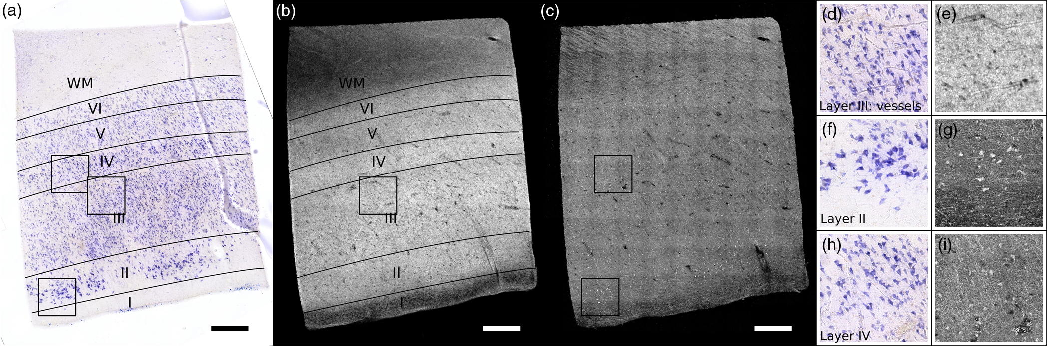 5.OCT AcquisitionAs shown in our previous publication,14 to obtain the overall laminar structure of the EC using the objective, the average intensity projection over in depth from the surface of each volume was performed, filtered,28,29 and intensity adjusted to enhance the contrast. The images were then stitched together to obtain the full cortical ribbon of the sample. Figure 1 shows the cortical layers in EC that are easily observable with OCT imaging [Fig. 1(b)] and corresponding Nissl [Fig. 1(a)]. Layers exhibit different intensities related to their cellular architecture and myelin content.30 To evaluate the capability of OCT to accurately resolve individual neurons, we performed high-resolution imaging on layers I–III in EC. The objective provides a depth of focus of about . Therefore, at each position of the sample, we acquired five volumes, every in depth, starting at under the surface until the first of the sample was imaged. The framed inset in Fig. 2 shows the depth schematic where the dashed lines represent the five different focus depths from which we acquired data. Contrary to what has been reported concerning freshly resected brain tissue or rodent brains23,24,31 where neurons exhibit a lack of backscattered light (shown as black spots in the images), neurons in ex vivo fixed human brain highly backscatter the light compared to the surrounding tissue, resulting in high intensity (white spots). Thus, for each of the five volumes, the maximum intensity projection (MIP) over around the focus plane (hatched regions around the focus planes) was performed to highlight the neurons. Each tile was then filtered and intensity adjusted. For each different depth, the tiles were acquired across the whole region of interest and were stitched using Fiji to provide the full FOV. Figure 1(d) shows an example of a high resolution OCT image corresponding to the Nissl stained slice and lower resolution OCT image. For the full cortical lamina, only one focus depth (, MIP over around the focus) was imaged and presented. Neurons of layers II and IV were visible, as shown in the inset of Figs. 1(g) and 1(i) and correspond to neurons observed on the Nissl stained slices [Figs. 1(f) and 1(h)]. Figures 2(a)–2(e) show the images obtained at the five different depths. Next, the five full images corresponding to each depth were stacked and the MIP in depth was performed to visualize all the neurons contained in the thick slices of the Nissl stained image. The resulting OCT image is shown in Fig. 2(f) and the corresponding Nissl stained slice in Fig. 2(g). The modular organization of layer II is clearly visible both in the OCT and the Nissl stained images. The dendrites arising from the neurons are visible on both images. However, on the OCT image, tangential fibers in layer I can also be observed. Fig. 2Images obtained of the same sample at five different focus depths (a-e). Dashed lines of the framed inset represent the different focus. The MIP was performed over the around the focus (dashed regions of the inset). (f) Composite image representing the neuron content over in depth and (g) the corresponding Nissl stained slice of section thickness. Scale bar: . 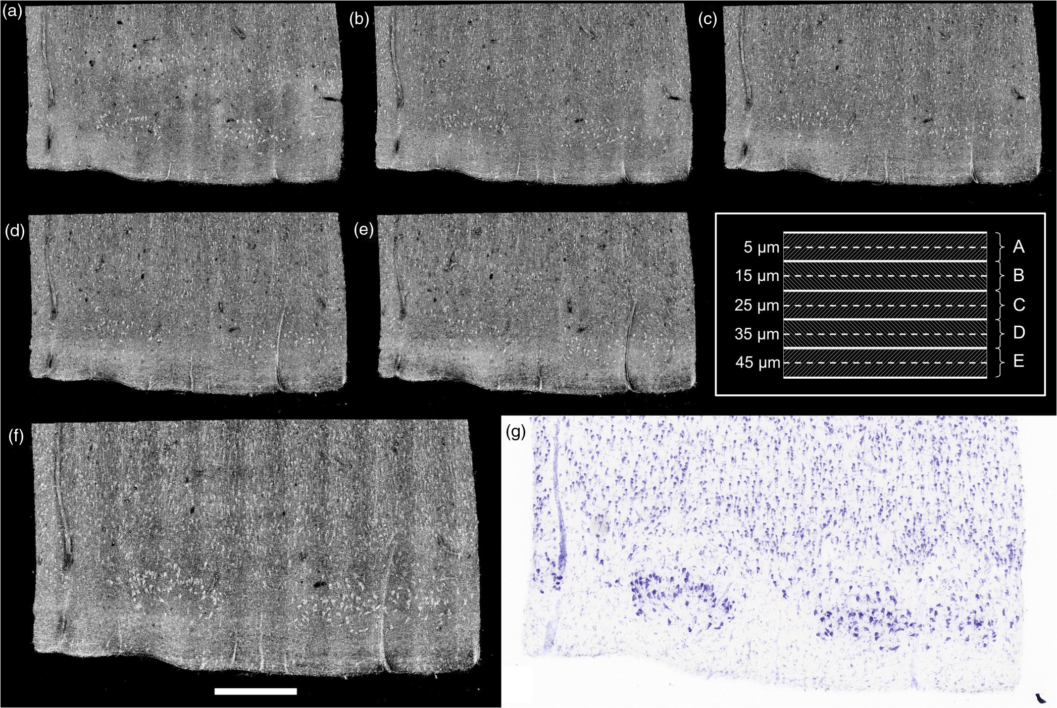 6.Registration and Segmentation of NeuronsTo assess the colocalization of the neurons between histologically stained slices and OCT images, the images were registered. Histology protocols can suffer from irretrievable distortions such as tears due to the sectioning, shrinking occurring during the drying process, and geometric warping during mounting. In spite of precautions taken to avoid distortions during the tissue processing, artifacts cannot be avoided completely in large human tissue samples. (For animal histology, these distortions can be reduced significantly using perfusion fixation, shorter PMIs and small samples.) For example, in Fig. 1(a) no outright tearing was observed, but note the vessel on the lower left corner. After mounting and drying in the Nissl protocol, the vessel left a gap, which stretched and locally shifted the location of neurons within the slice. OCT acquisition on the blockface does not suffer from such distortions since imaging occurs on the blockface prior to sectioning. A rigid registration is not sufficient to account for these distortions, therefore, we developed an in-house nonlinear registration tool. Corresponding landmarks on the Nissl stained and OCT images were manually selected, and a nonlinear transformation between the landmark points was computed based on the thin-plate splines32 deformation model using the implementation in the freely available ITK library (National Library of Medicine Insight Segmentation and Registration Toolkit).33 The computed transformation was applied to the Nissl-stained images, and the warped Nissl images were resampled by linear interpolation into the new coordinates. The accuracy of the registration algorithm with respect to the number of landmarks was then tested. A large number of corresponding neurons found on both modalities of tissue from Figs. 2(f) to 2(g) were manually selected (). Figure 3(a) shows the position of the cells on the OCT in green, and on the Nissl stain slice in blue, prior to nonlinear registration. In this example, the shrinkage due to drying and staining in Nissl is visible. landmarks were randomly selected to register the remaining points and the mean distance between the corresponding neurons was calculated. For each between 5 and 305, the procedure was repeated 100 times to estimate statistics on the distance error between the remaining corresponding landmarks. Figure 3(b) shows the registration results. The mean registration error is with selected landmarks, and quickly asymptotes to just over after 50 landmarks. Fig. 3(a) Neuron localization in OCT (green) and Nissl stain (blue) prior to registration. (b) Registration accuracy as a function of the number of landmark points. Note that the average error asymptotes to about after 50 landmarks, and is under after only 15 or so. 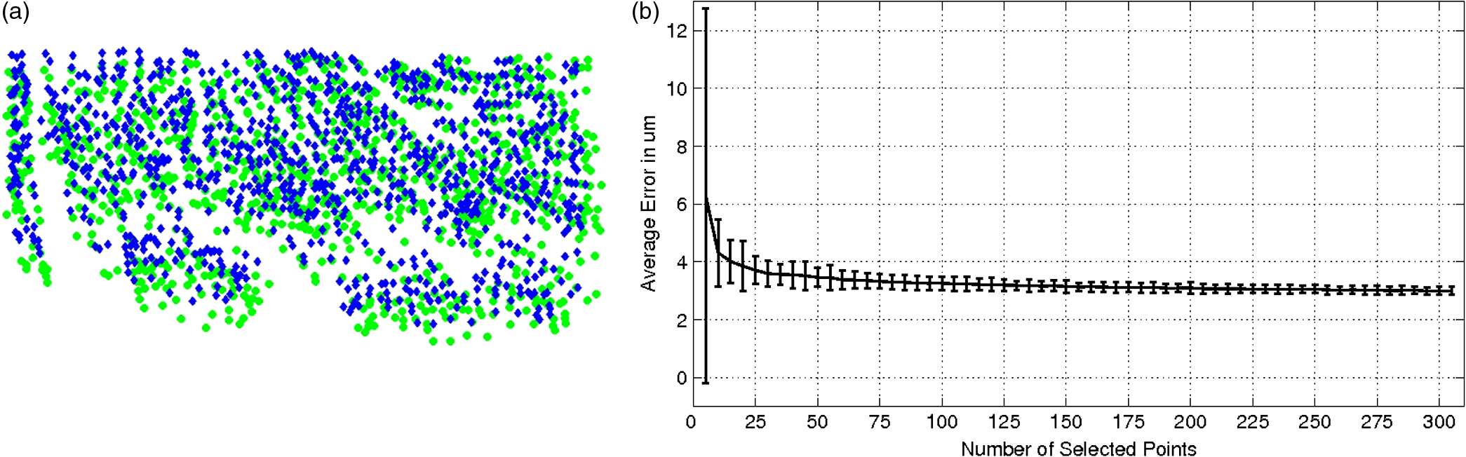 Next, the neurons were segmented. The neuronal segmentation in the Nissl-stained images was done using adaptive thresholding34 based on the implementation provided in the freely available OpenCV library.35 The thresholds used in the adaptive threshold at were the mean value of the neighborhood of minus a constant (, ) in Nissl-stained images. The segmentation was manually edited to add neurons whose contrast was insufficient to be identified automatically, and to remove glia and vessels that were segmented incorrectly. OCT images reveal more than just neurons. Vessels, dendrites, and possibly axons are also present in OCT images, for example, and exhibit the same kind of contrast. Moreover, the images are noisier than the Nissl stained slices. We first reduced the noise on each of the images obtained at the five different depths using a nonorthogonal wavelet algorithm optimized on a region of the image containing mainly noise (no visible neurons, fibers, or vessels).36 We then used adaptive thresholding ( and ) to segment the neurons. As we did for the Nissl stained slices, we manually edited each segmentation to remove nonneuronal features and to add missing neurons. Finally, those five segmentations were overlaid to generate the final OCT segmentation corresponding to the Nissl stained slice. 7.Results and DiscussionFigure 4 shows the registered Nissl stained slices (left panel), OCT images (center panel), and overlap of the segmented neurons found in layer II, delineated on the Nissl and OCT images by the lines (right panel) for the six tissue samples studied: green for Nissl, red for OCT, and yellow for the overlap. For each brain sample (A, B, and C), two slices were imaged, sectioned, and stained (1 and 2: two different slices from the same case). The agreement between the cytoarchitecture observed by the traditional Nissl stain and the OCT imaging appears excellent in case A, slice 1 (A1) and 2 (A2), good for slice B1 and case C (C1 and C2), and finally fair for B2. The agreement was visually assessed by CM. Looking closely at the overlay [Fig. 4 (left)], we can see that the shapes of the corresponding neurons are overall visually the same. However, a slight shift is often observed showing the limit of the registration between OCT images and histological slices that underwent multiple physical transformations (slicing, mounting, and drying). Fig. 4Colocalization of the neurons in layer II of EC for six different tissue samples: registered Nissl stain (left), OCT image (center), and the overlay of the segmented neurons (right): green for Nissl, red for OCT, and yellow for the overlap. Scale bar: . 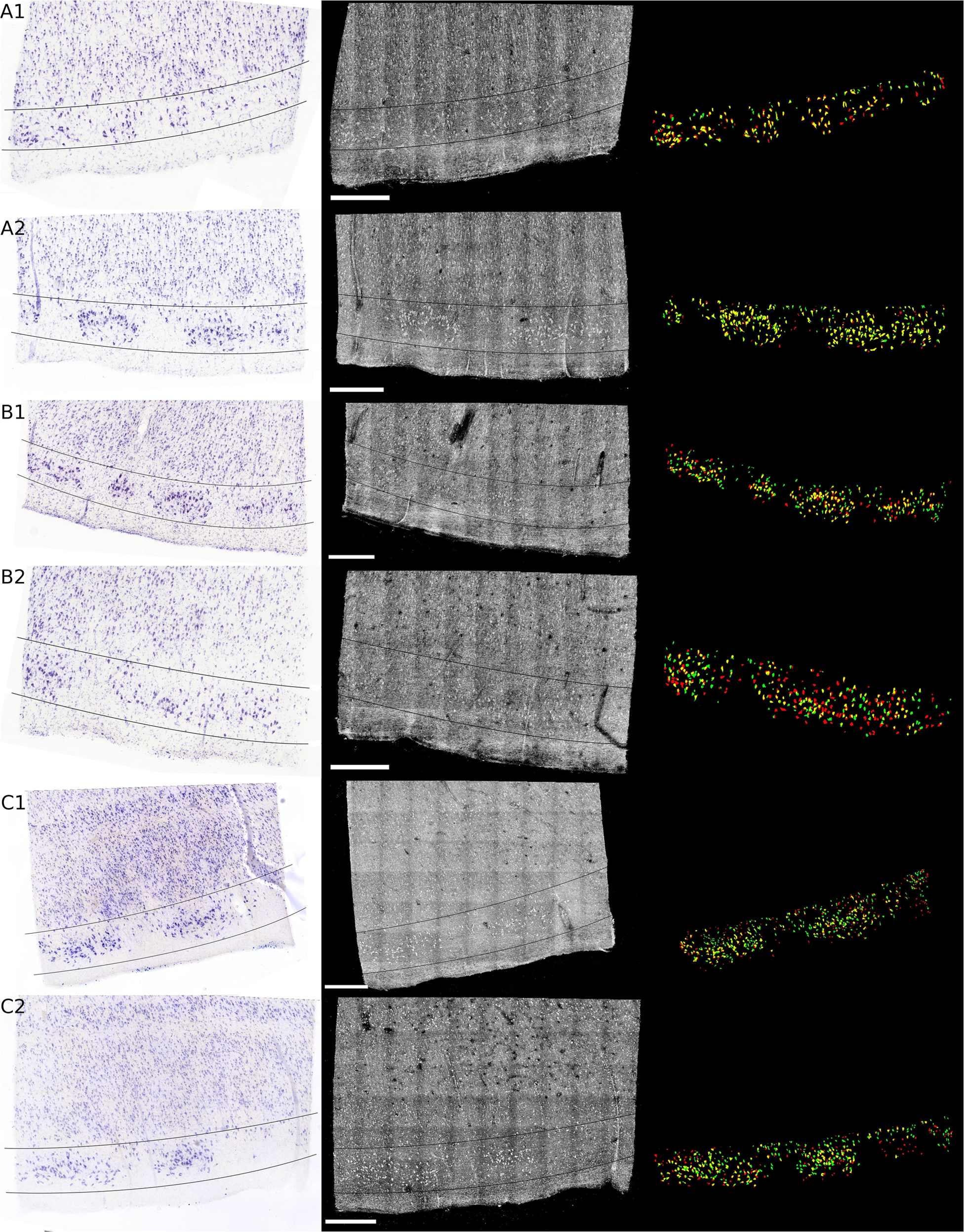 At least two possible reasons may explain the varied qualitative colocalization across samples. The first explanation lies in the registration of the Nissl stained slice to the OCT image, which depends on tissue integrity, sectioning, and mounting on the glass slides. All the slices but one (B2) were well prepared, with no major distortions observed and homogeneous tissue thickness. We observed that slice B2 was thinner on its right side. As a result, the density of neurons was lower on this side (Fig. 4). This thickness discrepancy within tissue is due to mispositioning of the sample with regard to the vibratome blade plane. In our present protocol, the vibratome is not yet integrated with the OCT rig and is a separate apparatus. The sample, once flatfaced, is moved to the OCT system for the acquisition and returned to the vibratome for the sectioning. When the sample is not placed exactly in the same position relative to the blade (difference in height and/or tilt occurs), the thickness is not uniform. In the future, the vibratome will be integrated with the OCT rig to remove this complication. The second explanation is the OCT imaging itself. Ideally, we focus the light at the depth of for the first image and then move the sample in increments until the first of the tissue is imaged, corresponding to the stained tissue. At the beginning of each experiment, we visually position the sample so that the light is focused at the surface and then the sample is moved up . Exact positioning of the sample is challenging since the axial pixel size is . After visually noting the discrepancy in the neuronal content agreement between modalities, we decided to evaluate the position of the light focus with respect to the surface. The surface and the focus planes were fitted by a third degree polynomial surface on every volume acquired at the five different focus depths on the region of interest (layer II). For the first theoretical depth (), the focus plane and the surface plane are too close to clearly differentiate them. We used the four subsequent theoretical depths to evaluate the experimental depth of focus and use a linear regression to assess the first experimental depth. Table 1 shows the results in the last column. Moreover, we used a built-in algorithm (bwlabel) in the MATLAB programming environment to count the number of neurons on the OCT segmentation image (binary image) obtained at the five different depths (neurons on OCT) and the number of those segmented neurons that are corresponding to neurons on the Nissl segmentation image (overlap on OCT). Finally, we used the same algorithm to assess the total number of neurons segmented on the final OCT segmentation (after overlaying the segmentation of the different depths) and the Nissl segmentation. For each slice, Table 1 reports the intended focus depth, the number of neurons on the OCT at that depth, the number of overlapping neurons, and the percentage of overlapping neurons normalized by the total number of neurons in OCT at each depth. Finally, we also noted the total neurons on OCT and Nissl staining in Table 1. The total number of neurons observed on the final image of OCT (for the ) is underestimated due to the presence of different neurons at different depths. It does not reflect the number of neurons we would obtain by adding the numbers of neurons at each depth. However, this total number of neurons is in excellent agreement with the number of neurons found on the Nissl stained images (with the exception of case B1, which will be explained in the next paragraph). Contrary to OCT, neurons at different depths cannot be differentiated automatically from the Nissl images—an important advantage of OCT. For case A, the focus position was good, between 8 and under the surface. The overlap between OCT and Nissl is above 69%. The overlap is a little lower for the last depth, which could be attributed to the slight mispositioning of the initial focus depth. Slice B1 shows a good overlap over the five different depths, over 70% even though the initial focus depth is about . The thickness of this slice was checked using a microscope (with Stereo Investigator, MBF Bioscience) and appears to be thicker than . This is confirmed by the fact that the total number of neurons found on the Nissl stained slices is about 1.5 time higher than the one reported on the OCT images. For the remaining slices, those numbers are comparable. B2 exhibits excellent overlap for the first two depths (over 90%), and a subsequent decrease for the next depths, explained by the deeper initial focus depth, around and the uneven sectioning (apparent tilt on the sample during the sectioning) of the tissue as discussed previously. Slices C1 and C2 show a good agreement also, the overlap being above 68% except for one depth. This discrepancy could be due to a false positive segmentation on the OCT images. Table 1Quantitative evaluation of the colocalization of the layer II neurons for each slice: number of neurons segmented on the OCT image with respect to the theoretical depth, number of neurons corresponding to neurons on the Nissl stain (overlap), percentage of the overlay, total number of neurons on the final OCT image (covering the 50 μm), and on the Nissl stained slice. The last columns show the actual depth of the first image.
8.Toward Neuropathology and Whole Brain ImagingEven though OCT does not have the molecular specificity of histology, this technique shows a variety of features, such as healthy neurons, vessels, and possibly axons as can be seen in the insets of Fig. 1. To assess the connectivity in the human brain more accurately, we will add polarization imaging to our OCM (polarization sensitive OCM) as shown in Wang et al.37,38 and obtain fiber orientation in addition to the backscatter contrast shown in this study. OCT may also be applicable to neuropathology, such as for the diagnosis of Alzheimer’s disease, traumatic brain injury, tumor,31 and cerebral amyloid angiopathy among others. For example, OCT can visualize amyloid plaques, as was shown in Bolmont et al.39 in a mouse model of Alzheimer’s disease. As shown in Fig. 4, each brain exhibits slightly different contrast when imaged by OCT depending on its contents. Case A very clearly shows the processes of the neurons, whereas case B is heavily myelinated (fibers running from WM to pial surface, as well as transversely). The automatic segmentation of these cortical features is a challenge that we are investigating. By improving and expanding our OCT system and postprocessing, larger brain regions can be imaged with minimal distortion. We have demonstrated that OCT can visualize neurons in depth by imaging at different focus planes under the tissue surface. To reduce the imaging time required to obtain volumetric data, an extended focus depth can be implemented both on the OCT setup itself by using a Bessel beam illumination40,41 or phase apodization,42 and in postprocessing by implementing digital refocusing.43–46 In the future, we plan on increasing the speed of data acquisition by using a camera with a 150 kHz scan rate (GL2048 from Sensors Unlimited). By coupling the vibratome to the OCT as suggested in Wang et al.,47 several cubic centimeters of tissues can be imaged with negligible distortion. The sectioning of the tissue will then be homogeneous and only dependent on the z-stage and the vibratome precision, which is better than .48 Detection of the focus depth will also be implemented in our acquisition software to control the initial position of the sample with respect to the light focus. 9.ConclusionIn this study, we showed that OCT can discriminate healthy neurons in ex vivo fixed human EC. This technique has been validated by the histological Nissl staining. The same of tissue was imaged by OCT and then stained with Nissl. The modalities were registered using a nonlinear transformation, neuronally segmented, and the overlap was quantified. The results showed good colocalization. Moreover, we demonstrate that OCT can discriminate the neurons in depth. In conclusion, we demonstrated that OCT/OCM is a promising technique to image the postmortem human brain at the level of single neurons. One critical advantage of OCT over Nissl staining is the minimal distortion of tissue, since the blockface tissue is imaged prior to sectioning. OCT paves the way to undistorted, high resolution, 3-D visualization of the cytoarchitecture in the human cortex. We anticipated that OCT can have a far-reaching impact in both basic neuroscience and clinical neuropathology. AcknowledgmentsWe acknowledge the National Center for Research Resources (P41-EB015896, U24 RR021382), the National Institute of Biomedical Imaging and Bioengineering (R01EB006758), the National Institute on Aging (AG022381, 5R01AG008122-22, K01AG028521, R01AG016495-11), the National Center for Alternative Medicine (RC1 AT005728-01), the National Institute for Neurological Disorders and Stroke (R01 NS052585-01, 1R21NS072652-01, 1R01NS070963), the Shared Instrumentation Grants (1S10RR023401, 1S10RR019307, 1S10RR023043) as well as The Autism & Dyslexia Project funded by the Ellison Medical Foundation, and by the NIH Blueprint for Neuroscience Research (5U01-MH093765), part of the multi-institutional Human Connectome Project. In addition, B.F. has a financial interest in CorticoMetrics, a company whose medical pursuits focus on brain imaging and measurement technologies. B.F. interests were reviewed and are managed by Massachusetts General Hospital and Partners HealthCare in accordance with their conflict of interest policies. ReferencesS. E. Arnold et al.,
“The topographical and neuroanatomical distribution of neurofibrillary tangles and neuritic plaques in the cerebral cortex of patients with Alzheimer’s disease,”
Cereb. Cortex, 1 103
–116
(1991). http://dx.doi.org/10.1093/cercor/1.1.103 53OPAV 1047-3211 Google Scholar
H. Braak and E. Braak,
“Neuropathological staging of Alzheimer-related changes,”
Acta Neuropathol., 82 239
–259
(1991). http://dx.doi.org/10.1007/BF00308809 ANPTAL 1432-0533 Google Scholar
P. V. Arriagada et al.,
“Neurofibrillary tangles but not senile plaques parallel duration and severity of Alzheimer’s disease,”
Neurology, 42 631
(1992). http://dx.doi.org/10.1212/WNL.42.3.631 NEURAI 0028-3878 Google Scholar
H. Braak and E. Braak,
“Staging of Alzheimer’s disease-related neurofibrillary changes,”
Neurobiol. Aging, 16
(3), 271
–278
(1995). http://dx.doi.org/10.1016/0197-4580(95)00021-6 NEAGDO 0197-4580 Google Scholar
T. Gomez-Isla et al.,
“Profound loss of layer II entorhinal cortex neurons occurs in very mild Alzheimer’s disease,”
J. Neurosci., 16
(14), 4491
–4500
(1996). JNRSDS 0270-6474 Google Scholar
H. Braak and E. Braak,
“Diagnostic criteria for neuropathologic assessment of Alzheimers disease,”
Neurobiol. Aging, 18 S85
–S88
(1997). http://dx.doi.org/10.1016/S0197-4580(97)00062-6 NEAGDO 0197-4580 Google Scholar
T. Gomez-Isla et al.,
“Neurond loss correlates with but exceeds neurofibrillary tangles in Alzheimer’s disease,”
Ann. Neurol., 41
(1), 17
–24
(1997). http://dx.doi.org/10.1002/(ISSN)1531-8249 ANNED3 0364-5134 Google Scholar
G. Simic et al.,
“Volume and number of neurons of the human hippocampal formation in normal aging and Alzheimers disease,”
J. Comp. Neurol., 379 482
–494
(1997). http://dx.doi.org/10.1002/(ISSN)1096-9861 JCNEAM 0021-9967 Google Scholar
K. Amunts et al.,
“BigBrain: an ultrahigh-resolution 3D human brain model,”
Science, 340 1472
–1475
(2013). http://dx.doi.org/10.1126/science.1235381 SCIEAS 0036-8075 Google Scholar
J. C. Augustinack et al.,
“Direct visualization of the perforant pathway in the human brain with ex vivo diffusion tensor imaging,”
Front. Hum. Neurosci., 4 42
(2010). http://dx.doi.org/10.3389/fnhum.2010.00042 Google Scholar
C. Ceritoglu et al.,
“Large deformation diffeomorphic metric mapping registration of reconstructed 3D histological section images and in vivo MR images,”
Front. Hum. Neurosci., 4 43
(2010). http://dx.doi.org/10.3389/fnhum.2010.00043 Google Scholar
M. Reuter, H. D. Rosas and B. Fischl,
“Highly accurate inverse consistent registration: a robust approach,”
Neuroimage, 53 1181
–1196
(2010). http://dx.doi.org/10.1016/j.neuroimage.2010.07.020 NEIMEF 1053-8119 Google Scholar
M. Reuter et al.,
“Registration of histology and MRI using blockface as intermediate space,”
(2012). Google Scholar
C. Magnain et al.,
“Blockface histology with optical coherence tomography: a comparison with Nissl staining,”
Neuroimage, 84 524
–533
(2014). http://dx.doi.org/10.1016/j.neuroimage.2013.08.072 NEIMEF 1053-8119 Google Scholar
W. Denk, J. H. Strickler and W. W. Webb,
“2-photon laser scanning fluorescence microscopy,”
Science, 248
(4951), 73
–76
(1990). http://dx.doi.org/10.1126/science.2321027 SCIEAS 0036-8075 Google Scholar
P. T. C. So et al.,
“Two-photon excitation fluorescence microscopy,”
Annu. Rev. Biomed. Eng., 2 399
–429
(2000). http://dx.doi.org/10.1146/annurev.bioeng.2.1.399 ARBEF7 1523-9829 Google Scholar
F. Helmchen and W. Denk,
“Deep tissue two-photon microscopy,”
Nat. Methods, 2
(12), 932
–940
(2005). http://dx.doi.org/10.1038/nmeth818 1548-7091 Google Scholar
T. Ragan et al.,
“Serial two-photon tomography for automated ex vivo mouse brain imaging,”
Nat. Methods, 9 255
–258
(2012). http://dx.doi.org/10.1038/nmeth.1854 1548-7091 Google Scholar
S. W. Oh et al.,
“A mesoscale connectome of the mouse brain,”
Nature, 508 207
–214
(2014). http://dx.doi.org/10.1038/nature13186 NATUAS 0028-0836 Google Scholar
K. Chung et al.,
“Structural and molecular interrogation of intact biological systems,”
Nature, 497 332
–337
(2013). http://dx.doi.org/10.1038/nature12107 NATUAS 0028-0836 Google Scholar
D. Huang et al.,
“Optical coherence tomography,”
Science, 254
(5035), 1178
–1181
(1991). http://dx.doi.org/10.1126/science.1957169 SCIEAS 0036-8075 Google Scholar
V. J. Srinivasan et al.,
“Optical coherence microscopy for deep tissue imaging of the cerebral cortex with intrinsic contrast,”
Opt. Express, 20 2220
–2239
(2012). http://dx.doi.org/10.1364/OE.20.002220 OPEXFF 1094-4087 Google Scholar
C. Leahy, H. Radhakrishnan and V. J. Srinivasan,
“Volumetric imaging and quantification of cytoarchitecture and myeloarchitecture with intrinsic scattering contrast,”
Biomed. Opt. Express, 4 1978
–1990
(2013). http://dx.doi.org/10.1364/BOE.4.001978 BOEICL 2156-7085 Google Scholar
F. Li et al.,
“Nondestructive evaluation of progressive neuronal changes in organotypic rat hippocampal slice cultures using ultrahigh-resolution optical coherence microscopy,”
Neurophotonics, 1 025002
(2014). http://dx.doi.org/10.1117/1.NPh.1.2.025002 NEUROW 2329-423X Google Scholar
J. B. Arous et al.,
“Single myelin fiber imaging in living rodents without labeling by deep optical coherence microscopy,”
J. Biomed. Opt., 16 116012
(2011). http://dx.doi.org/10.1117/1.3650770 JBOPFO 1083-3668 Google Scholar
M. S. Islam et al.,
“Extracting structural features of rat sciatic nerve using polarization-sensitive spectral domain optical coherence tomography,”
J. Biomed. Opt., 17
(5), 056012
(2012). http://dx.doi.org/10.1117/1.JBO.17.5.056012 JBOPFO 1083-3668 Google Scholar
S. Preibisch, S. Saalfeld and P. Tomancak,
“Globally optimal stitching of tiled 3D microscopic image acquisitions,”
Bioinformatics, 25 1463
–1465
(2009). http://dx.doi.org/10.1093/bioinformatics/btp184 BOINFP 1367-4803 Google Scholar
G. Gilboa, N. Sochen and Y. Y. Zeevi,
“Texture preserving variational denoising using an adaptive fidelity term,”
in Proc. Variational, Geometric and Level Set Methods in Computer Vision,
137
–144
(2003). Google Scholar
S. Monica et al.,
“Nonlinear total variation based noise removal algorithms,”
Physica D, 60
(1–4), 259
–268
(1992). http://dx.doi.org/10.1016/0167-2789(92)90242-F PDNPDT 0167-2789 Google Scholar
J. C. Augustinack et al.,
“MRI parcellation of ex vivo medial temporal lobe,”
Neuroimage, 93 252
–259
(2013). Google Scholar
O. Assayag et al.,
“Imaging of non-tumorous and tumorous human brain tissues with full-field optical coherence tomography,”
Neuroimage, 2 549
–557
(2013). http://dx.doi.org/10.1016/j.nicl.2013.04.005 NEIMEF 1053-8119 Google Scholar
F. L. Bookstein,
“Principal warps: thin-plate and the decomposition of deformations,”
IEEE Trans. Pattern Anal. Mach. Intell., 11
(6), 567
–585
(1989). http://dx.doi.org/10.1109/34.24792 ITPIDJ 0162-8828 Google Scholar
T. S. Yoo et al.,
“Engineering and algorithm design for an image processing Api: a technical report on ITK—the insight Toolkit,”
Stud. Health Technol. Inf., 85 586
–592
(2002). SHTIEW 0926-9630 Google Scholar
R. Gonzales and R. E. Woods, Digital Image Processing, 3rd ed.Prentice-Hall, Inc., Upper Saddle River, New Jersey
(2006). Google Scholar
G. Bradski,
“The opencv library,”
Doctor Dobbs J., 25
(11), 120
–126
(2000). 1044-789X Google Scholar
M. Gargesha et al,
“Denoising and 4D visualization of OCT images,”
Opt. Express, 16
(16), 12313
–12333
(2008). http://dx.doi.org/10.1364/OE.16.012313 OPEXFF 1094-4087 Google Scholar
H. Wang et al.,
“Reconstructing micrometer-scale fiber pathways in the brain: multi-contrast optical coherence tomography based tractography,”
Neuroimage, 58 984
–992
(2011). http://dx.doi.org/10.1016/j.neuroimage.2011.07.005 NEIMEF 1053-8119 Google Scholar
H. Wang et al.,
“Cross-validation of serial optical coherence scanning and diffusion tensor imaging: a study on neural fiber maps in human medulla oblongata,”
Neuroimage, 100 395
–404
(2014). http://dx.doi.org/10.1016/j.neuroimage.2014.06.032 NEIMEF 1053-8119 Google Scholar
T. Bolmont et al.,
“Label-free imaging of cerebral -amyloidosis with extended-focus optical coherence microscopy,”
J. Neurosci., 32
(42), 14548
–14556
(2012). http://dx.doi.org/10.1523/JNEUROSCI.0925-12.2012 JNRSDS 0270-6474 Google Scholar
Z. Ding et al.,
“High-resolution optical coherence tomography over a large depth range with an axicon lens,”
Opt. Lett., 27 243
–245
(2002). http://dx.doi.org/10.1364/OL.27.000243 OPLEDP 0146-9592 Google Scholar
R. A. Leitgeb et al.,
“Extended focus depth for Fourier domain optical coherence microscopy,”
Opt. Lett., 31 2450
–2452
(2006). http://dx.doi.org/10.1364/OL.31.002450 OPLEDP 0146-9592 Google Scholar
L. Liu et al.,
“Binary-phase spatial filter for real-time swept-source optical coherence microscopy,”
Opt. Lett., 32 2375
–2377
(2007). http://dx.doi.org/10.1364/OL.32.002375 OPLEDP 0146-9592 Google Scholar
T. S. Ralston et al.,
“Inverse scattering for optical coherence tomography,”
J. Opt. Soc. Am. A, 23 1027
–1037
(2006). http://dx.doi.org/10.1364/JOSAA.23.001027 JOAOD6 0740-3232 Google Scholar
Y. Yasuno et al.,
“Three-dimensional line-field Fourier domain optical coherence tomography for in vivo dermatological investigation,”
J. Biomed. Opt., 11
(1), 014014
(2006). http://dx.doi.org/10.1117/1.2166628 JBOPFO 1083-3668 Google Scholar
T. S. Ralston et al.,
“Interferometric synthetic aperture microscopy,”
Nat. Phys., 3 129
–134
(2007). http://dx.doi.org/10.1038/nphys514 NPAHAX 1745-2473 Google Scholar
L. Yu et al.,
“Three-dimensional angle measurement based on propagation vector analysis of digital holography,”
Appl. Opt., 46
(17), 3539
–3545
(2007). http://dx.doi.org/10.1364/AO.46.003539 APOPAI 0003-6935 Google Scholar
S. Wang et al.,
“Three-dimensional computational analysis of optical coherence tomography images for the detection of soft tissue sarcomas,”
J. Biomed. Opt., 19 021102
(2014). http://dx.doi.org/10.1117/1.JBO.19.2.021102 JBOPFO 1083-3668 Google Scholar
T. Ragan et al.,
“High-resolution whole organ imaging using two-photon tissue cytometry,”
J. Biomed. Opt., 12
(1), 014015
(2007). http://dx.doi.org/10.1117/1.2435626 JBOPFO 1083-3668 Google Scholar
BiographyCaroline Magnain received her PhD degree in 2009 from the Université Pierre et Marie Curie, Paris 6, France, for her work on skin color modeling and its representation in works of art. She is a postdoctoral fellow in the Athinoula A. Martinos Center for Biomedical Imaging at Massachusetts General Hospital, Harvard Medical School. Her current research focuses on optical coherence tomography applied to the human brain structure and connectivity. Jean C. Augustinack obtained her PhD degree in neuroanatomy and cell biology at the University of Iowa and is now an assistant professor in radiology at Massachusetts General Hospital, Harvard Medical School. Her research is centered on two main concentrations: brain mapping and neuropathological systems in Alzheimer’s disease. Ender Konukoglu received his PhD degree in computer science from Sophia Antipolis and the University of Nice, France. He is now an instructor in the Radiology Department at Massachusetts General Hospital, Harvard Medical School. His research is focused on biomedical image analysis, vision for medical and biological applications, machine learning, and mathematical modeling. Matthew P. Frosch received his undergraduate degree in chemistry (summa cum laude) from Amherst College and his MD and PhD degrees in biophysics from Harvard University. He was trained in anatomic pathology and neuropathology at Brigham and Women’s Hospital and was a Paul B. Beeson Faculty Scholar in Aging Research from 1999 to 2002. Van J. Wedeen, MD, is an associate professor in radiology at Harvard Medical School, assistant neuroscientist at Massachusetts General Hospital, and director of Connectomics at Martinos Center, Department of Radiology, Massachusetts General Hospital. His present work is focused on discovery with diffusion MRI of new aspects of geometric order in the CNS, including complex path coherence within the cerebral cortex, and organization of cerebral white matter and connectivity across multiple scales. David A. Boas is a PhD physicist and professor of radiology at Massachusetts General Hospital, Harvard Medical School. He has published more than 150 peer-reviewed papers in the field of biomedical optics. He is the founding editor-in-chief of Neurophotonics. |
||||||||||||||||||||||||||||||||||||||||||||||||||||||||||||||||||||||||||||||||||||||||||||||||||||||||||||||||||||||||||||||||||||||||||||||||||||||||||


