Correspondence of electroencephalography and near-infrared spectroscopy sensitivities to the cerebral cortex using a high-density layout

Paolo Giacometti; Solomon G. Diamond

doi:10.1117/1.NPh.1.2.025001

2 September 2014 Correspondence of electroencephalography and near-infrared spectroscopy sensitivities to the cerebral cortex using a high-density layout

Paolo Giacometti, Solomon G. Diamond

Author Affiliations +

Neurophotonics, Vol. 1, Issue 2, 025001 (September 2014). https://doi.org/10.1117/1.NPh.1.2.025001

Abstract

This study investigates the correspondence of the cortical sensitivity of electroencephalography (EEG) and near-infrared spectroscopy (NIRS). EEG forward model sensitivity to the cerebral cortex was calculated for 329 EEG electrodes following the 10-5 EEG positioning system using a segmented structural magnetic resonance imaging scan of a human subject. NIRS forward model sensitivity was calculated for the same subject using 156 NIRS source-detector pairs selected from 32 source and 32 detector optodes positioned on the scalp using a subset of the 10-5 EEG positioning system. Sensitivity correlations between colocalized NIRS source-detector pair groups and EEG channels yielded R=0.46±0.08 . Groups of NIRS source-detector pairs with maximum correlations to EEG electrode sensitivities are tabulated. The mean correlation between the point spread functions for EEG and NIRS regions of interest (ROI) was R=0.43±0.07 . Spherical ROIs with radii of 26 mm yielded the maximum correlation between EEG and NIRS averaged across all cortical mesh nodes. These sensitivity correlations between EEG and NIRS should be taken into account when designing multimodal studies of neurovascular coupling and when using NIRS as a statistical prior for EEG source localization.

1. Introduction

Electroencephalography (EEG) studies aim to gain insight into the mechanisms of brain function and the effects of disease, age, therapy, and medication on the brain. EEG measures the electric potentials on the scalp that are generated by neural source currents.¹ The interpretation of EEG measurements relies on knowledge of the correspondence between the scalp coordinates of the EEG electrodes used to record the signal and the underlying anatomical and functional regions of the cortex.²^,³ Similarly, near-infrared spectroscopy (NIRS) measures hemodynamics associated with functional brain activity that arises from changes in blood oxygenation and blood volume in the area of activation.⁴ The interpretation of NIRS signals also relies on knowledge of the correspondence of scalp measurements and the underlying brain regions.

In the brain, there are complex subsystems composed of neurons, capillaries, astrocytes, and microglia, that are referred to as neurovascular units.⁵ The components within these neurovascular units function in intricate ways to maintain the homeostasis in the brain. The functional connection between neural activity and hemodynamics mediated by the neurovascular unit is referred to as neurovascular coupling. It is important to understand the neurovascular coupling to gain greater insight into the physiology of brain function and to ascertain what constitutes normal or pathological neurovascular coupling in a healthy brain compared with the one that suffers from disease.⁶ Neurovascular coupling decline could be a significant factor in neurodegenerative diseases as it has been observed in disorders such as Alzheimer’s disease, hypertension, and ischemic stroke.⁵^–⁷ In addition to providing further knowledge regarding brain function, studies of neurovascular coupling aim to yield new metrics for the diagnosis and treatment of neurodegenerative diseases.⁸^,⁹

In order to study the neurovascular coupling, multimodal neuroimaging systems that measure neural and vascular signals are required. A multimodal neuroimaging approach is typically used, such as integrating EEG with functional magnetic resonance imaging (fMRI),¹⁰ magnetoencephalography (MEG) with NIRS,¹¹ or EEG with NIRS.¹² Combining EEG and NIRS is particularly advantageous because of the comparatively low cost and portability of these systems in contrast to other imaging systems such as magnetic resonance imaging (MRI), MEG, or positron emission tomography. Multimodal studies, such as those that combine EEG and NIRS, examine the combined neurovascular origins of the brain activation signals. In such studies, interpretation of the data for EEG and NIRS can be done independently for the signals measured from each system, or concurrently, to understand the relationship between the signals during the period of activation. Analyzing neurovascular coupling information provided by the neural activity measured with EEG and the hemodynamic activity measured with NIRS requires that the signals measured by each system originate from the same activated regions of the brain. The sensitivity correspondence between the two modalities is what allows the spatial and temporal relationship between the signals to be studied.

Sensitivity maps for source localization analysis can be computed from the EEG and NIRS forward models. These sensitivity maps are often computed when analyzing the signals of the EEG and NIRS independently.¹³^–¹⁶ The inverse of the forward model can be used to compute tomographic maps of the cortical activity. Joint reconstructions of the cortical activity often rely on statistical priors that apply the appropriate weighting between NIRS and EEG data.¹⁷^,¹⁸ Interpretation of EEG data can be improved upon and the number of electrodes needed for measurement can be reduced by using NIRS hemodynamic responses as statistical priors.¹⁸

In this study, we computed the forward and inverse models for EEG and NIRS and calculated their correspondence to help with analysis and interpretation of multimodal studies. The forward models were computed for both systems by drawing from 329 scalp positions following the 10-5 EEG positioning system, which is an extension of the 10-20 International EEG positioning system.² Then, the intersection and correlation of the sensitivity to the brain for both systems were analyzed. The inverse models for both EEG and NIRS were computed from their corresponding forward model solutions. Correlations between the inverse models were computed for the whole cortical surface and for the regions of interest (ROI) distributed throughout the cortical surface. The results are discussed in terms of the correspondence of the brain regions to EEG, NIRS, and their intersection. Also, the influence of the correlation between EEG and NIRS signals on neurovascular coupling studies is discussed.

1.1.

EEG Forward Model

The neural activity measured by EEG is generated by millions of neurons firing in spatial and temporal synchrony. Focal neural activity is often modeled as a current dipole in the cerebral cortex.¹ Electric potentials from neural currents can be measured at the surface of the scalp with EEG electrodes. The EEG forward problem simulates the distribution of electric potentials at locations on the scalp where EEG electrodes are placed that result from current dipoles in the cortex, assuming infinite impedance between the electrode and the scalp.¹⁹^–²¹ The electric potential distribution on the scalp generated by the dipoles depends on the orientation of the dipole, so the forward model simulation must account for the cortical folds of gyri and sulci. The solution to the forward model is obtained using the quasistatic solution to the Maxwell equations in a conducting medium, which is the Poisson equation

Eq. (1)

\nabla \cdot (σ \nabla V) = f = \nabla \cdot J,

where

σ

[(Ω m^{- 1})]

is the tissue conductivity within the region,

V

(V) is the electric potential,

f

is the electric dipole source, and the divergence of the current source density is

J

(A / m^{2})

.¹^,²² The resulting forward model formulation yields a linear relationship between the scalp potentials

V

and the current dipoles

J

. There are several methods to compute the forward model such as using a boundary element mesh (BEM) method or a finite element method using a tetrahedral mesh. These two methods require anatomical segmentations from a MRI structural scan to generate either boundary or volume meshes of the different tissues in the head such as the scalp, skull, cerebrospinal fluid (CSF), and white and gray matter. For each electrode position, the forward model is a distribution of the contribution of each current dipole to the electric potential measured at that electrode, in units of

V / (A m)

.²¹

1.2.

NIRS Forward Model

The NIRS forward model accounts for the transport of light that is illuminated onto the head from optode source locations on the scalp, migration of light through the head tissues, and re-emission at the scalp locations of the optode detectors. The propagation of light in tissue is modeled throughout the head volume using the radiative transport equation (RTE).²³^,²⁴ The RTE is an expression for conservation of radiance over a controlled volume

Eq. (2)

\frac{1}{c_{m}} \cdot \frac{\partial L (r, t, \hat{s})}{\partial t} + \nabla \cdot \hat{s} L (r, t, \hat{s}) = - μ_{t} L (r, t, \hat{s}) + μ_{s} \int_{4 π} L (r, t, \hat{s}) f_{ph} (\hat{s}, {\hat{s}}^{'}) d ω^{'} + S (r, t, \hat{s}),

where

c_{m}

(m / s^{2})

is the speed of light in the medium, and

L (r, t, \hat{s})

({Wm}^{- 2} {sr}^{- 1})

is the radiance in position

r

, at time

t

, and direction

\hat{s}

. The total attenuation coefficient

μ_{t}

(m^{- 1})

is the sum of the absorption coefficient

μ_{a}

(m^{- 1})

and the scattering coefficient

μ_{s}

(m^{- 1})

. The term

(1 / c_{m}) \cdot [\partial L (r, t, \hat{s})] / \partial t

in the RTE is the rate of change of the radiance, or the difference between the photons entering and leaving the volume;

\nabla \cdot \hat{s} L (r, t, \hat{s})

is the flux of radiance out of the volume;

- μ_{t} L (r, t, \hat{s})

accounts for the losses of radiance due to absorption and scattering;

μ_{s} \int_{4 π} L (r, t, \hat{s}) f_{ph} (\hat{s}, {\hat{s}}^{'}) d ω^{'}

accounts for the corresponding radiance gains where

f_{ph} (\hat{s}, {\hat{s}}^{'})

is the normalized differential scattering phase function, or the probability that a photon traveling in direction

{\hat{s}}^{'}

will be scattered toward direction

\hat{s}

; and

S (r, t, \hat{s})

({Wm}^{- 3} {sr}^{- 1})

is a source term that accounts for irradiance on the tissue or fluorescence within the tissue. In the case of NIRS, the source term is the light illuminated by the optode source.⁴

The forward model is computed from a perturbation of the system modeled by the RTE in the form of localized small changes in the optical properties. Specifically, the effects of small changes in the absorption coefficient can be modeled as the linear relationship provided by the modified Beer Lambert law that relates optical density and light intensity measurements²⁵^,²⁶

Eq. (3)

Δ OD = - \log_{10} (\frac{I_{s d, t_{2}}}{I_{s d, t_{1}}}) = ε_{λ} Δ [C] 〈 L 〉,

where

Δ OD

is the change in optical density, and

I_{s d, t}

is the light intensity from the source s measured at the detector d at time t.⁴ The forward model

F

relates the measured light intensity to the changes in chromophore concentration

Δ [C]

. The forward model is specified by the mean optical pathlength

〈 L 〉

, which is the average distance that the photons travel from entering the tissue from the optode sources until being scattered back toward the detector at the surface and is weighted by the wavelength-dependent molar extinction coefficient of the tissue

ε_{λ}

as

Eq. (4)

F = 〈 L 〉 \cdot ε_{λ}, 〈 L 〉 = ζ L_{s d},

where

F

is the forward model and

ζ

is the differential pathlength factor, which relates the mean optical pathlength to the distance

L_{s d}

between the source and the detector for each pair. Optical properties of tissue, such as the extinction coefficient, are often given in terms of the absorption coefficient

μ_{a}

, since they are directly related by

Eq. (5)

μ_{a} = \ln (10) ε_{λ} [C] .

Therefore, given tissue absorption coefficients, source and detector scalp coordinates, the forward model provides a direct way of obtaining tomographic reconstructions of chromophore concentration changes in the brain from light intensity measurements. The forward model represents the sensitivity of each NIRS channel to the chromophore changes of interest. NIRS channels correspond to source-detector pairs rather than individual detectors as NIRS measurements require both a source and a detector. Although the forward model is often computed in order to generate the inversion and the tomographic reconstructions of the chromophore concentrations, the forward model alone provides a lot of information for NIRS studies of the human head. The sensitivity matrix resulting from the forward model calculation provides information about the extent of the head that is examined with NIRS, what regions of the brain are investigated, and the effect of other tissues on the NIRS signal measured.¹⁶^,²⁷

A common method for calculating the forward model is to use a Monte Carlo technique to simulate the light transport of photons through the tissues. An alternative method of simulating the forward model is to use the diffusion approximation to the RTE instead of simulation.⁴^,²⁸ The diffusion approximation is accurate except when modeling light transport through the CSF layer, which is a very low-scattering medium.²⁹^–³¹ The Monte Carlo simulations of the RTE account for the low-scattering CSF regions and thus yield more accurate results.

1.3.

EEG and NIRS Inverse Models

The EEG forward model linearly relates the current dipole sources in the cortex to the EEG measurements obtained at the electrode locations on the scalp. The dipole source strengths can be estimated from measured EEG data by inverting the forward model. The EEG inverse model specifies the linear relationship between the EEG measurements $V$ and the dipole sources $J$ . The NIRS forward model specifies the linear relationship between the tissue optical properties and the NIRS measurements obtained at the optode locations on the scalp. Similar to the EEG inverse model, the NIRS inverse model relates the changes in optical density to localized changes in the optical properties of the tissue. Inverting EEG and NIRS forward models is generally an ill-posed problem and requires the application of several specialized techniques.³²^–³⁴

2. Methods

2.1.

EEG Forward Model

The sensitivity of the brain to the EEG electrodes was computed for 329 electrodes from an EEG forward model solution using the 10-5 positioning system.²^,³⁵ To compute an EEG forward model, surface meshes of the head tissues, tissue conductivities, and EEG electrode positions are required. A simulated adult human MRI structural scan was obtained from BrainWeb, a publicly available database of head tissue segmentations, and simulated T1 images using a SFLASH (spoiled FLASH) sequence with $T R = 22 ms$ , $T E = 9.2 ms$ , a 30 deg flip angle, and 1 mm isotropic voxel size, generated from real-MRI head scans obtained under IRB approval.³⁶^,³⁷ Freesurfer (Athinoula A. Martinos Center for Biomedical Imaging, Cambridge, Massachusetts) and Brainstorm (documented and freely available for download online under the GNU general public license)³⁸ were used to segment the MRI head scan into four BEM surfaces (scalp, skull, CSF, and brain) and to calculate the EEG forward model. The process involved several steps.

First, Freesurfer was used to segment the cortical surface from the MRI head scan in order to obtain a BEM.¹⁶^,³⁵^,³⁹^–⁴² Then, the MRI head scan and the segmented cortical BEM were loaded into Brainstorm. The scalp surface was segmented from the MRI using the Brainstorm function “Generate head surface.” Using the scalp and brain surfaces, BEMs of the outer and inner sides of the skull were generated with a 4-mm skull thickness using the “Generate BEM Surfaces” function. The scalp BEM was then exported to MATLAB, where an EEG electrode positioning algorithm was used to calculate 329 electrode scalp coordinates using the 10-5 positioning system.³⁵ Those positions were then imported back into Brainstorm. The scalp, outer skull, inner skull, and cortex BEM surfaces were used in conjunction with the 10-5 EEG scalp coordinates to compute the forward model, using the Open MEEG routine.²¹^,²² The forward model was computed using tissue conductivity ratios of 1 for the CSF/brain regions, 0.0125 for the skull/CSF regions, and 1 for the scalp/skull regions.²⁰^,²² The air/scalp region ratio was set to 0 because air was assumed to be nonconductive. The electrical conductivity for each tissue type was assumed to be uniform within each region. Dipole sources were placed at each node of the brain BEM surface. The BEM method was used to calculate the forward model for the electrode positions placed on the scalp. The BEM surfaces used had 1082 nodes for the scalp, 642 for the outer skull, 642 for the inner skull, and 325,987 for the brain. The matrix resulting from the computation contained gain values for each node in the brain BEM for the $x$ , $y$ , and $z$ directions for each electrode. To compute the EEG sensitivity for each electrode, the gain values at each node were projected along the local directional vector that is normal to the cortical surface

Eq. (6)

S_{n, e} = G_{n, e} \cdot r_{n},

where

S_{n, e}

is the sensitivity of electrode e to brain mesh node n,

G

is the gain, and

r

is the node directional vector.

The contrast-to-noise ratio (CNR) was computed for the EEG forward model analysis in order to select the sensitivity above the noise floor. The CNR was computed from the sensitivity for each node and electrode $S_{n, e}$ , using an instrument noise of $1.0 μ V_{rms}$ , a signal activation of 0.2 pAm per pyramidal neuron, and a volume of activation of 200,000 synchronized neurons.⁴³^,⁴⁴ The sensitivity of EEG was set to zero for all nodes with CNR values under 0 dB.

2.2.

EEG Inverse Model

The matrix formulation of the EEG forward model $S$ , obtained from Eq. (1), is

Eq. (7)

V = S J,

relating the scalp potentials

V

and the current dipoles

J

. The inverse model

M

was computed from the forward model

S

using a Bayesian approach

Eq. (8)

M_{EEG} = {Γ S}^{T} {(S Γ S^{T} + Λ)}^{- 1},

where

Γ

is the signal covariance matrix prior and

Λ

is the noise covariance matrix. The EEG inverse model solution

M_{EEG}

was calculated from the sensitivity matrix

S

, using the Brainstorm function “Compute Sources” which uses the

L_{2}

-minimum norm estimation algorithm from Eq. (8).⁴⁵ The noise covariance matrix was calculated from the ratio of instrument noise covariance and signal covariance using the same noise and signal activation as the EEG CNR calculations described in Sec. 2.1. The result is an inverted matrix with dimensions of the number of cortical nodes by the number of EEG electrode channels.

2.3.

NIRS Forward Model

In this study, we computed the NIRS forward model for a human head using the tetrahedral mesh of a head segmented into four regions: scalp, skull, CSF, and brain. A Monte-Carlo simulation method was used to illuminate photons into the mesh at locations specified by the EEG 10-5 positioning system, using tissue optical properties commonly used in the field. The matrix formulation of the NIRS forward model is

Eq. (9)

Δ OD = F Δ [C],

which relates

Δ OD

from Eq. (3) to the NIRS forward model

F

and the change in chromophore concentrations

Δ [C]

.⁴

The sensitivity of the brain to each NIRS detector was computed for 64 optodes (32 sources and 32 detectors) as a NIRS forward model solution using a subset of the 10-5 EEG positioning system. The layout of the optode sources and detectors, and the 156 optode pairings selected, is illustrated in Fig. 1. The NIRS forward model was computed using mesh-based Monte Carlo (MMC) (Athinoula A. Martinos Center for Biomedical Imaging, Cambridge, Massachusetts),⁴⁶which is a software tool for simulation of the RTE for light propagation in tissue. The simulation computes the trajectory and weight of millions of individual photons as they propagate through tissue undergoing absorption and scattering events. Photon re-emission at the detector locations is also tracked. The software generates a matrix of fluence $(1 / {mm}^{2})$ at each tetrahedral mesh node for each time step of the period specified.

Fig. 1

Electrode and optode layouts and source-detector pair schematic. Note: Only 65 electrodes are displayed (10-10 positioning system) for the illustration purposes only. Also, source-detector distances are not representative of true separation.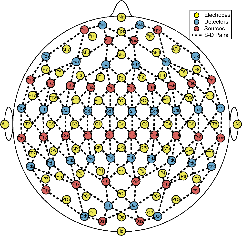

The BEM surfaces used for the EEG forward model were exported onto MATLAB. MMC requires tetrahedral volume meshes instead of the triangular BEMs used for the EEG forward model computation. The complexity of the brain BEM made it impossible to maintain the 325,987 nodes at the surface when converting to a tetrahedral mesh. To avoid that issue, we computed the convex hull that envelopes each hemisphere of the brain. The surface meshes of the scalp, outer skull, inner skull, and left and right hemispheres of the brain were converted to a single-head mesh of 52,662 nodes, 300,742 tetrahedral elements, and multiple regions using the iso2mesh (Athinoula A. Martinos Center for Biomedical Imaging, Cambridge, Massachusetts)⁴⁷ package function “surf2mesh.” MMC also requires that the source optode positions be inside of a tetrahedral element. Since the 10-5 scalp coordinates lie on the surface of the head rather than inside it, the centroid of the tetrahedral element closest to each position was chosen as the source optode position. This shifted the positions by an average of $2.04 \pm 0.7 mm$ , which altered the source-detector separations by an average of $0.45 \pm 1.39 mm$ without affecting the results. A single simulation was computed with 10 million photons for each position for a time period of 5 ns using 0.1 ns time steps. The simulations were performed using a uniform refractive index $η$ of 1.37, a uniform anisotropy coefficient $g$ of 0.89, and the optical properties listed in Table 1.²⁷^,⁴⁷^–⁴⁹

Table 1

Tissue optical properties.

Tissue type	Absorption coefficient $μ_{a}$ $({mm}^{- 1})$	Anisotropy coefficient $g$ (no units)	Scattering coefficient $μ_{s}$ $({mm}^{- 1})$	Reduced scattering coefficient $μ_{s}^{'}$ $({mm}^{- 1})$
Scalp	0.0170	0.89	7.8	0.858
Skull	0.0116	0.89	7.8	0.858
CSF	0.004	0.89	0.009	0.001
Brain	0.0178	0.89	9.1	1.0

Note: The reduced scattering coefficient (μs′) combines the scattering coefficient (μs) and the anisotropy coefficient (g) as μs′=(1−g)μs.

The sensitivity of NIRS was computed for each of the 156 source-detector pairs that are marked in Fig. 1. The positions chosen follow the layout of the NIRS–EEG head probe developed by our lab.⁵⁰ The source-detector pairs chosen have a mean separation distance of $42.30 \pm 7.48 mm$ , as shown in Fig. 2. Although the source-detector pairs chosen yielded larger separations than those commonly used for analysis, a CNR threshold of 0 dB was used in the analysis to give less weight to channels with larger distances. The CNR variance for each channel is plotted against the channel source-detector distance in Fig. 2.

Fig. 2

(a) Histogram of source-detector pair separation distances. (b) Contrast-to-noise ratio (CNR) variance ( ${CNR}_{var}$ ) for each source-detector pair versus its corresponding separation distance.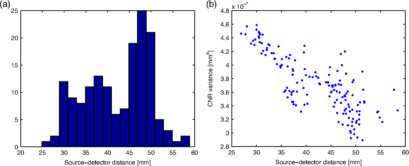

The results of the Monte Carlo simulations need to be further processed in order to obtain a sensitivity matrix. The result of each simulation was a value of fluence ( $Φ$ ) at each node of the tetrahedral head mesh for the 50 time steps simulated. The mean transit time ${\bar{t}}_{tr}$ was calculated for each source-detector pair selected as

Eq. (10)

{\bar{t}}_{tr} = \frac{\sum_{i} t_{i} \cdot Φ_{s, t_{i}} (r_{d})}{\sum_{i} Φ_{s, t_{i}} (r_{d})},

where

t_{i}

is the simulation time at step

i

, and

Φ_{s, t_{i}} (r_{d})

is the fluence at time step

t_{i}

from the source s at position

r_{d}

of detector d. The mean transit time calculated for all selected source-detector pairs was

1.03 \pm 0.15 ns

. From the mean transit time, the mean optical pathlength

〈 L 〉

was calculated as

Eq. (11)

〈 L 〉 = {\bar{t}}_{tr} \cdot \frac{c}{η},

where

c / η

is the speed of light

c

in tissue with index of refraction

η

. The mean optical pathlength for all source-detector pairs chosen was

22.5 \pm 3.2 cm

. Finally, for each source-detector pair, the differential pathlength factor

ζ

was calculated from the mean optical pathlength and the distance between the source and detector

L_{s d}

. To ensure accuracy, the mean transit time, mean optical pathlength, and differential pathlength factor were calculated from the fluence simulated at the source and at the detector positions, using the source-detector pair and the detector-source pair, and then averaging them. The differential pathlength factor for all source-detector pairs had a mean value of

ζ = 5.37 \pm 0.44

.

To compute the NIRS sensitivity matrix, the fluence was summed over time to obtain the total fluence during the simulation, yielding a matrix of fluence for each node by each source optode position. The sensitivity $A_{p} (r_{n})$ of each source-detector pair p for each node at position $r_{n}$ was calculated from the fluence fields as

Eq. (12)

A_{p} (r_{n}) = \frac{Φ_{s} (r_{n}) Φ_{d} (r_{n})}{Φ_{s} (r_{d})},

where

Φ_{s} (r_{n})

is the fluence from source s at nodal position

r_{n}

,

Φ_{d} (r_{n})

is the fluence from detector d at nodal position

r_{n}

, and

Φ_{s} (r_{d})

is the fluence from source s at detector position

r_{d}

. A normalization factor

N_{F}

was calculated for the sensitivity of each source-detector pair to account for the source-detector separation distance as

Eq. (13)

N_{F} = \frac{〈 L 〉}{\sum_{j} A_{p} (v_{j}) \cdot V_{j}}, A_{p} (v) = {\bar{A}}_{p} (r_{n 1}, r_{n 2}, r_{n 3}, r_{n 4}),

where

A_{p} (v_{j})

is the volume sensitivity for tetrahedral element

j

and source-detector pair p, calculated as the average sensitivity at each node of the tetrahedron (

r_{n 1}

,

r_{n 2}

,

r_{n 3}

, and

r_{n 4}

), and

V_{j}

is the volume of the tetrahedral element

j

. The normalized sensitivity

A^{†} (r)

for each source-detector pair was calculated as the sensitivity multiplied by its corresponding normalization factor. Since the normalization factor included the fluence at each nodal position, normalizing the sensitivity yielded a matrix with the form of a mean optical pathlength per unit volume at each node with units of (

mm / {mm}^{3} \to 1 / {mm}^{2}

), the same units as the original fluence field.

Since our aim was to compare the NIRS forward model against the EEG forward model, the sensitivity was needed at each brain BEM mesh node rather than at the head tetrahedral mesh nodes. To obtain those values, a linear three-dimensional (3-D) interpolation was computed for all values of the sensitivity at all nodal positions. From the interpolation, the sensitivity values corresponding to the nodes of the BEM were computed, yielding a sensitivity matrix equal in size to the EEG sensitivity matrix for each NIRS source-detector pair.

The CNR was computed for the NIRS sensitivity matrix in order to select values above the noise floor. The number of photons $N_{ph}$ detected at each electrode was computed as

Eq. (14)

N_{ph} = \frac{Φ^{†} P_{i} F_{c}^{2}}{f_{s} \cdot E_{ph}}, Φ^{†} = \frac{Φ_{s} (r_{d})}{Φ_{s} (r_{s})},

where

P_{i}

is the incident power of the system, set at 5 mW,

F_{c}

is the optical coupling loss factor, set at 50%,

f_{s}

is the sampling frequency, set at 200 Hz,

E_{ph}

is the energy of a photon, calculated using the wavelength of the laser source set at

808 nm

, and

Φ^{†}

(no units) is the normalized detected fluence, which was computed from the ratio of the fluence from the source at the detector position

Φ_{s} (r_{d})

and the fluence from the source at the source position

Φ_{s} (r_{s})

.¹⁶^,⁵¹ The shot noise

N_{s}

was calculated as the square root of the number of photons detected

N_{s} = \sqrt{N_{ph}}

. The instrument noise

N_{i}

was computed as

Eq. (15)

N_{i} = \frac{P_{n e} \cdot \sqrt{f_{s}}}{f_{s} \cdot E_{ph}},

where the noise equivalent power

P_{ne}

was set to

0.05 pW / {Hz}^{1 / 2}

. The measurement noise

N_{m}

(no units) for the detected fluence was computed as

Eq. (16)

N_{m} = \sqrt{N_{s}^{2} + N_{i}^{2}} .

The change in optical density from measurement noise was computed for each source-detector pair p as

Eq. (17)

N_{p} = \ln [\frac{Φ^{†} + N_{m}}{Φ^{†}}] .

Finally, the CNR was computed for each source-detector pair at each node in dB as

Eq. (18)

CNR = 20 \cdot \log_{10} [\frac{A^{†} (r) \cdot v_{act} \cdot \partial μ_{a}}{N_{p}}],

for an assumed volume of brain activation of

v_{act} = 5 \cdot 5 \cdot 5 {mm}^{3}

accompanied by a change in absorption coefficient

\partial μ_{a} = 0.0001 {mm}^{- 1}

. The normalized sensitivity

A^{†} (r)

was set to zero for nodes with CNR values below 0 dB for each source-detector pair.¹⁶^,⁵¹

2.4.

NIRS Inverse Model

The NIRS forward model can be inverted such that the changes in chromophore concentrations can be computed directly from light intensity measurements as

Eq. (19)

Δ [C] = M_{NIRS} Δ OD,

where

M_{NIRS}

is the inverse model for NIRS, calculated in the same way as was done for EEG using Eq. (8), but substituting the EEG sensitivity matrix

S

with the normalized NIRS sensitivity

A^{†}

. The NIRS noise covariance matrix for this calculation was obtained from the ratio of the noise covariance and the signal covariance,

Eq. (20)

{CNR}_{var} = \frac{{(v_{act} \cdot \partial μ_{a})}^{2}}{N_{p}^{2}} .

Figure 2 shows the CNR variance ( ${CNR}_{var}$ ) used to weight each channel with respect to their corresponding source-detector separation, so that channels with larger separations have less influence on the analysis results. Tomographic calculations can be made using this method to transform linear NIRS measurements into diffuse optical tomography reconstructions of brain activity in the form of chromophore concentration changes or blood volume changes.⁴

2.5.

NIRS–EEG Sensitivity Correlation

The NIRS-EEG head probe electrode and optode layout was followed to select the NIRS source-detector pair sensitivities and electrode sensitivities such that each electrode corresponds spatially with an optode pair, as shown in Fig. 1. The area of the brain to which an EEG electrode is maximally sensitive is underneath the electrode, whereas the area to which a NIRS source-detector pair is maximally sensitive lies in the region between the source and the detector. Because of this, the colocation of EEG and NIRS channels does not correspond to colocalized EEG electrodes and NIRS optodes but rather to EEG electrodes and NIRS source-detector pairs. Spatially colocating electrode positions and the midpoint of source-detector distances attempts to maximize the simultaneous monitoring of the same brain regions using EEG and NIRS. The correlation $R_{e, p}$ of EEG and NIRS sensitivities was computed as

Eq. (21)

R_{e, p} = \frac{\sum_{n} S_{e, n} \cdot A_{p, n}^{�}}{\sqrt{\sum_{n} {(S_{e, n})}^{2} \cdot \sum_{n} {(A_{p, n}^{�})}^{2}}},

where

S_{e, n}

is the EEG sensitivity from electrode e to brain mesh node n, and

A_{p, n}^{†}

is the NIRS normalized sensitivity from source-detector pair p to node n. The resulting correlation matrix has the size of the number of electrodes by the number of source-detector pairs.

Optimal groups of source-detector pairs that maximally correlated with each electrode were obtained using the following steps. First, the correlation matrix $R$ was sorted from maximum to minimum correlations with respect to each electrode. The sorted matrix yielded the source-detector channels in descending order of correlation with each individual electrode. Next, groups of NIRS source-detectors were selected based on the sorted results. The first group was the sensitivity of the pair with the highest correlation to one electrode; the second group was the combined sensitivity of the pairs with the highest and the second highest correlations to the same electrode; the third group was the combined sensitivity of the pairs with the three highest correlations to the same electrode; this same process was carried out for the top 30 pairs and for all 329 electrodes. So, for each electrode, group g was computed as the sum of the sensitivities of the first $k$ source-detector pairs with the highest correlation with that electrode. The grouping yielded a new NIRS sensitivity matrix that, instead of having the size of the 156 NIRS channels, had the same size as the EEG sensitivity matrix (329 channels). Then, new correlations were computed for each group of source-detector pairs’ sensitivity and their corresponding electrode sensitivity. The result was a correlation matrix with the size of electrodes by the 30 groups of source-detector pairs. Finally, the group that had the highest correlation for each electrode was selected as the optimal group for that electrode, yielding a set $R_{e, g, \max}$ with a single-correlation value for each electrode e and group of source-detector pairs g. The number of group calculations (30) we performed was to ensure that we reached the maximum correlation in all cases to find the optimal group. In reality, most optimal groups had significantly fewer pairs per group and required fewer calculations.

A reference table of optimal source-detector pair groupings with respect to each electrode was also generated, containing one source-detector pair group for each electrode that correlated maximally. A subset of 65 EEG electrode positions, corresponding to the 10-10 positioning layout, was chosen from the 329 positions for displaying the tabulated results in order to follow the layout of the NIRS-EEG head probe we use in our lab.⁵⁰ The electrodes selected for Table 2 are indicated in Fig. 1.

Table 2

Optimal source-detector pair groups for each EEG channel. Calculations were made for 65 selected EEG positions based on the 10-10 EEG positioning layout. The EEG position corresponding to each source and detector position is labeled in parentheses. Source-detector pair groupings were thresholded at k=4 pairs. The correlation between the thresholded source-detector groups and their corresponding electrode has a mean value of R=0.44±0.08.

EEG position	Source-detector pair 1(EEG position)	Source-detector pair 2(EEG position)	Source-detector pair 3(EEG position)	Source-detector pair 4(EEG position)
Nz	Fps1 (AFp1)–Fpd2 (NFp2h)	Fps2 (AFp2)–Fpd2 (NFp2h)	Fps2 (AFp2)–Fpd1 (NFp1h)	Fps1 (AFp1)–Fpd1 (NFp1h)
Fp1	Fps1 (AFp1)–Fpd1 (NFp1h)	Fps1 (AFp1)–Fd7 (AFF5)	Fps3 (AFp9h)–Fd7 (AFF5)	Fps3 (AFp9h)–Fpd1 (NFp1h)
Fpz	Fps1 (AFp1)–Fpd2 (NFp2h)	Fps2 (AFp2)–Fpd1 (NFp1h)	Fps2 (AFp2)–Fpd2 (NFp2h)	Fps1 (AFp1)–Fpd1 (NFp1h)
Fp2	Fps2 (AFp2)–Fpd2 (NFp2h)	Fps2 (AFp2)–Fd8 (AFF6)	Fps4 (AFp10h)–Fpd2 (NFp2h)	Fps4 (AFp10h)–Fd8 (AFF6)
AF7	Fps3 (AFp9h)–Fd7 (AFF5)	—	—	—
AF3	Fps1 (AFp1)–Fd7 (AFF5)	Fps1 (AFp1)–Fd3 (AFF1)	Fps3 (AFp9h)–Fd7 (AFF5)	Fs5 (FFC5h)–Fd3 (AFF1)
AFz	Fps2 (AFp2)–Fd3 (AFF1)	Fps1 (AFp1)–Fd4 (AFF2)	Fps1 (AFp1)–Fd3 (AFF1)	Fps2 (AFp2)–Fd4 (AFF2)
AF4	Fps2 (AFp2)–Fd8 (AFF6)	Fps2 (AFp2)–Fd4 (AFF2)	Fs4 (FFC4h)–Fd8 (AFF6)	Fps1 (AFp1)–Fd4 (AFF2)
AF8	Fps4 (AFp10h)–Fd8 (AFF6)	Fs10 (FFT10h)–Fd8 (AFF6)	—	—
F7	Fs7 (FFT7h)–Fd9 (AFF9h)	Fs9 (FFT9h)–Fd7 (AFF5)	—	—
F5	Fs7 (FFT7h)–Fd7 (AFF5)	Fs5 (FFC5h)–Fd7 (AFF5)	Fs9 (FFT9h)–Fd7 (AFF5)	Fs3 (FFC3h)–Fd7 (AFF5)
F3	Fs5 (FFC5h)–Fd3 (AFF1)	Fs3 (FFC3h)–Fd7 (AFF5)	—	—
F1	Fs1 (FFC1h)–Fd3 (AFF1)	Fs3 (FFC3h)–Fd3 (AFF1)	Fs2 (FFC2h)–Fd3 (AFF1)	Fs5 (FFC5h)–Fd3 (AFF1)
Fz	Fs2 (FFC2h)–Fd3 (AFF1)	Fs1 (FFC1h)–Fd4 (AFF2)	Fs1 (FFC1h)–Fd3 (AFF1)	Fs2 (FFC2h)–Fd4 (AFF2)
F2	Fs2 (FFC2h)–Fd4 (AFF2)	Fs4 (FFC4h)–Fd4 (AFF2)	Fs6 (FFC6h)–Fd4 (AFF2)	Fs1 (FFC1h)–Fd4 (AFF2)
F4	Fs4 (FFC4h)–Fd8 (AFF6)	Fs6 (FFC6h)–Fd4 (AFF2)	—	—
F6	Fs8 (FFT8h)–Fd8 (AFF6)	Fs6 (FFC6h)–Fd8 (AFF6)	Fs10 (FFT10h)–Fd8 (AFF6)	Fs4 (FFC4h)–Fd8 (AFF6)
F8	Fs8 (FFT8h)–Fd10 (AFF10h)	Fs10 (FFT10h)–Fd8 (AFF6)	—	—
FT7	Fs9 (FFT9h)–Td7 (FTT7h)	Fs7 (FFT7h)–Td9 (FTT9h)	Fs7 (FFT7h)–Td7 (FTT7h)	Ts9 (TTP9h)–Td7 (FTT7h)
FC5	Fs5 (FFC5h)–Td7 (FTT7h)	Fs7 (FFT7h)–Cd5 (FCC5h)	—	—
FC3	Fs3 (FFC3h)–Cd5 (FCC5h)	Fs5 (FFC5h)–Cd3 (FCC3h)	—	—
FC1	Fs3 (FFC3h)–Cd1 (FCC1h)	Fs1 (FFC1h)–Cd3 (FCC3h)	Fs1 (FFC1h)–Cd1 (FCC1h)	Fs3 (FFC3h)–Cd3 (FCC3h)
FCz	Fs2 (FFC2h)–Cd1 (FCC1h)	Fs1 (FFC1h)–Cd2 (FCC2h)	Fs2 (FFC2h)–Cd2 (FCC2h)	Fs1 (FFC1h)–Cd1 (FCC1h)
FC2	Fs2 (FFC2h)–Cd4 (FCC4h)	Fs4 (FFC4h)–Cd2 (FCC2h)	Fs2 (FFC2h)–Cd2 (FCC2h)	—
FC4	Fs4 (FFC4h)–Cd6 (FCC6h)	Fs6 (FFC6h)–Cd4 (FCC4h)	—	—
FC6	Fs6 (FFC6h)–Td8 (FTT8h)	Fs8 (FFT8h)–Cd6 (FCC6h)	Fs8 (FFT8h)–Td8 (FTT8h)	Fs6 (FFC6h)–Cd6 (FCC6h)
FT8	Fs8 (FFT8h)–Td10 (FTT10h)	Fs10 (FFT10h)–Td8 (FTT8h)	—	—
T9	Ts9 (TTP9h)–Td9 (FTT9h)	Ts9 (TTP9h)–Td7 (FTT7h)	Ts9 (TTP9h)–Pd9 (TPP9h)	Ts7 (TTP7h)–Td9 (FTT9h)
T7	Ts9 (TTP9h)–Td7 (FTT7h)	Ts7 (TTP7h)–Td9 (FTT9h)	Ts7 (TTP7h)–Td7 (FTT7h)	Fs9 (FFT9h)–Td7 (FTT7h)
C5	Cs5 (CCP5h)–Td7 (FTT7h)	Ts7 (TTP7h)–Cd5 (FCC5h)	Cs5 (CCP5h)–Cd5 (FCC5h)	Ts7 (TTP7h)–Td7 (FTT7h)
C3	Cs5 (CCP5h)–Cd3 (FCC3h)	Cs3 (CCP3h)–Cd5 (FCC5h)	—	—
C1	Cs1 (CCP1h)–Cd3 (FCC3h)	Cs3 (CCP3h)–Cd1 (FCC1h)	—	—
Cz	Cs1 (CCP1h)–Cd2 (FCC2h)	Cs2 (CCP2h)–Cd1 (FCC1h)	Cs2 (CCP2h)–Cd2 (FCC2h)	Cs1 (CCP1h)–Cd1 (FCC1h)
C2	Cs4 (CCP4h)–Cd2 (FCC2h)	Cs2 (CCP2h)–Cd4 (FCC4h)	—	—
C4	Cs4 (CCP4h)–Cd6 (FCC6h)	Cs6 (CCP6h)–Cd4 (FCC4h)	—	—
C6	Ts8 (TTP8h)–Cd6 (FCC6h)	Cs6 (CCP6h)–Td8 (FTT8h)	—	—
T8	Ts10 (TTP10h)–Td8 (FTT8h)	Ts8 (TTP8h)–Td10 (FTT10h)	—	—
T10	Ts10 (TTP10h)–Td10 (FTT10h)	Ts10 (TTP10h)–Td8 (FTT8h)	Ts10 (TTP10h)–Pd10 (TPP10h)	Ts8 (TTP8h)–Td10 (FTT10h)
TP7	Ts9 (TTP9h)–Pd7 (TPP7h)	Ts7 (TTP7h)–Pd9 (TPP9h)	—	—
CP5	Cs5 (CCP5h)–Pd7 (TPP7h)	Ts7 (TTP7h)–Pd5 (CPP5h)	Ts7 (TTP7h)–Pd7 (TPP7h)	Cs5 (CCP5h)–Pd5 (CPP5h)
CP3	Cs5 (CCP5h)–Pd3 (CPP3h)	Cs3 (CCP3h)–Pd5 (CPP5h)	Cs3 (CCP3h)–Pd3 (CPP3h)	Cs5 (CCP5h)–Pd5 (CPP5h)
CP1	Cs1 (CCP1h)–Pd3 (CPP3h)	Cs3 (CCP3h)–Pd1 (CPP1h)	—	—
CPz	Cs1 (CCP1h)–Pd2 (CPP2h)	Cs2 (CCP2h)–Pd1 (CPP1h)	Cs1 (CCP1h)–Pd1 (CPP1h)	Cs2 (CCP2h)–Pd2 (CPP2h)
CP2	Cs4 (CCP4h)–Pd2 (CPP2h)	Cs2 (CCP2h)–Pd4 (CPP4h)	Cs2 (CCP2h)–Pd2 (CPP2h)	Cs4 (CCP4h)–Pd4 (CPP4h)
CP4	Cs4 (CCP4h)–Pd6 (CPP6h)	Cs6 (CCP6h)–Pd4 (CPP4h)	Cs4 (CCP4h)–Pd4 (CPP4h)	Cs6 (CCP6h)–Pd6 (CPP6h)
CP6	Ts8 (TTP8h)–Pd6 (CPP6h)	Cs6 (CCP6h)–Pd8 (TPP8h)	Ts8 (TTP8h)–Pd8 (TPP8h)	Cs6 (CCP6h)–Pd6 (CPP6h)
TP8	Ts10 (TTP10h)–Pd8 (TPP8h)	Ts8 (TTP8h)–Pd10 (TPP10h)	—	—
P7	Ps9 (PPO9h)–Pd7 (TPP7h)	Ps7 (PPO5)–Pd9 (TPP9h)	—	—
P5	Ps7 (PPO5)–Pd7 (TPP7h)	Ps7 (PPO5)–Pd5 (CPP5h)	Ps7 (PPO5)–Pd3 (CPP3h)	Ps7 (PPO5)–Pd9 (TPP9h)
P3	Ps7 (PPO5)–Pd3 (CPP3h)	Ps3 (PPO1)–Pd5 (CPP5h)	—	—
P1	Ps3 (PPO1)–Pd3 (CPP3h)	Ps3 (PPO1)–Pd1 (CPP1h)	Ps3 (PPO1)–Pd5 (CPP5h)	Ps3 (PPO1)–Pd2 (CPP2h)
Pz	Ps3 (PPO1)–Pd2 (CPP2h)	Ps4 (PPO2)–Pd1 (CPP1h)	Ps3 (PPO1)–Pd1 (CPP1h)	Ps4 (PPO2)–Pd2 (CPP2h)
P2	Ps4 (PPO2)–Pd4 (CPP4h)	Ps4 (PPO2)–Pd2 (CPP2h)	Ps4 (PPO2)–Pd6 (CPP6h)	Ps4 (PPO2)–Pd1 (CPP1h)
P4	Ps8 (PPO6)–Pd4 (CPP4h)	Ps4 (PPO2)–Pd6 (CPP6h)	Ps8 (PPO6)–Pd6 (CPP6h)	Ps4 (PPO2)–Pd4 (CPP4h)
P6	Ps8 (PPO6)–Pd6 (CPP6h)	Ps8 (PPO6)–Pd8 (TPP8h)	Ps8 (PPO6)–Pd10 (TPP10h)	Ps8 (PPO6)–Pd4 (CPP4h)
P8	Ps10 (PPO10h)–Pd8 (TPP8h)	Ps8 (PPO6)–Pd10 (TPP10h)	—	—
PO7	Ps7 (PPO5)–Od3 (POO9h)	Ps9 (PPO9h)–Od3 (POO9h)	Ps7 (PPO5)–Pd9 (TPP9h)	Ps7 (PPO5)–Od1 (POO1)
PO3	Ps7 (PPO5)–Od1 (POO1)	—	—	—
POz	Ps4 (PPO2)–Od1 (POO1)	Ps3 (PPO1)–Od2 (POO2)	Ps4 (PPO2)–Od2 (POO2)	—
PO4	Ps8 (PPO6)–Od2 (POO2)	—	—	—
PO8	Ps8 (PPO6)–Od4 (POO10h)	—	—	—
O1	Os1 (OI1h)–Od1 (POO1)	Os1 (OI1h)–Od3 (POO9h)	Ps7 (PPO5)–Od3 (POO9h)	Ps7 (PPO5)–Od1 (POO1)
Oz	Os1 (OI1h)–Od1 (POO1)	Os2 (OI2h)–Od1 (POO1)	Os1 (OI1h)–Od2 (POO2)	Os2 (OI2h)–Od2 (POO2)
O2	Ps8 (PPO6)–Od4 (POO10h)	Os2 (OI2h)–Od4 (POO10h)	Ps8 (PPO6)–Od2 (POO2)	Os2 (OI2h)–Od2 (POO2)
Iz	Os1 (OI1h)–Od2 (POO2)	Os1 (OI1h)–Od1 (POO1)	Os2 (OI2h)–Od2 (POO2)	Os2 (OI2h)–Od1 (POO1)

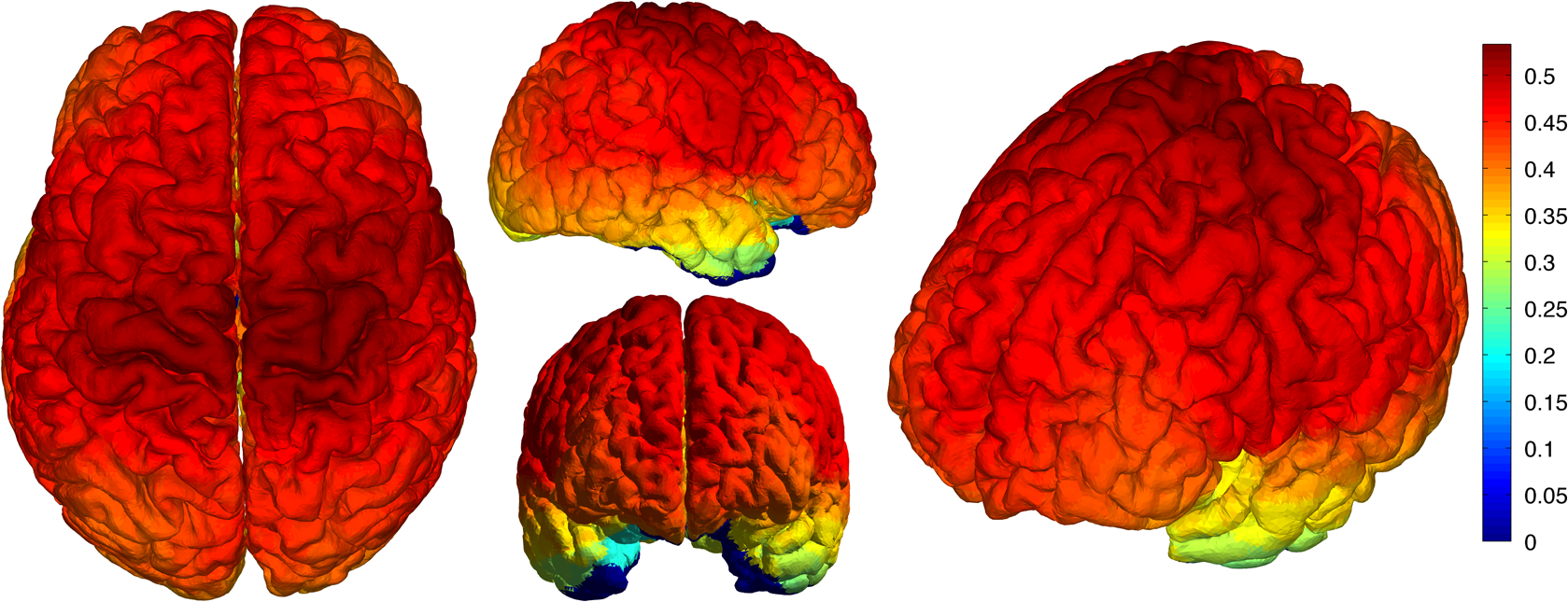
2.6.

NIRS-EEG Inverse Model Correlation

The correspondence of the EEG and NIRS inverse models was computed for all nodes in the cortex. For each cortical node, a point spread function (PSF) was obtained across all EEG channels by multiplying the sensitivity of that node to all electrode channels by the EEG inverse model. This calculation was repeated for the NIRS forward and inverse models, yielding a PSF for each brain mesh node for both EEG and NIRS. A NIRS-EEG correlation value was calculated for each cortical mesh node from the correlation of the PSFs centered at that given cortical mesh node; the value of the PSF for each brain mesh node for both EEG and NIRS was set to zero for all nodes with CNR values under 0 dB. The diagram in Fig. 3 illustrates the process to calculate the NIRS-EEG correlation at each brain mesh node. The PSF for EEG and NIRS at each node was calculated as the product of the forward model $F$ at node $i$ for all channels by the inverse model $M$ as

Eq. (22)

{PSF}_{i} = F_{i} M .

Fig. 3

Method for calculation of nodal point spread function (PSF) correlation. (a) Selection of brain mesh node. (b) Near-infrared spectroscopy (NIRS) PSF for selected node. (c) Electroencephalography (EEG) PSF for selected node. (d) Correlation of $R = 0.7$ between EEG ( $x$ -axis) and NIRS ( $y$ -axis) PSFs at selected node (normalized units).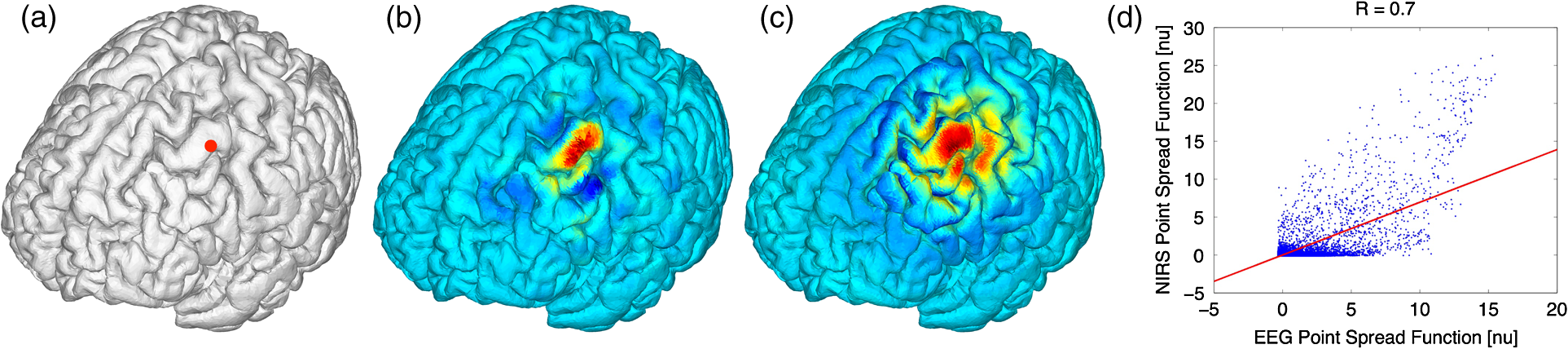

The PSF at the node shows the distribution of reconstructed activity from a point source at node $i$ for each system as seen in Fig. 3(b) for NIRS and in Fig. 3(c) for EEG. The calculation of the correlation is visually represented in Fig. 3(d) as the slope of the regression line between the two distributions plotted against each other.

Lastly, a ROI analysis was performed for the correspondence of the EEG and NIRS inverse models. An EEG positioning algorithm was used to calculate the evenly subdivided 3-D coordinates of 329 positions on the surface of the scalp following the 10-5 positioning system.³⁵ The scalp coordinates were then projected onto the cortical surface. To do this, a plane was fit to the set of cortical mesh nodes closest to each scalp position, as shown in blue in Fig. 4(a). Then, the normal to the plane (blue) that connects with each scalp coordinate (green point in space) was calculated. Finally, the projection point was calculated as the intersection point (red point on surface) between the plane normal and the triangular mesh element on the surface of the cortex. This method yielded 329 evenly distributed positions on the surface of the cortical mesh.

Fig. 4

(a) Method for the projection of scalp coordinates onto the surface of the cortex. (a1) Plane is fit to set of cortical mesh nodes (blue). (a2) Normal to plane (blue) that crosses scalp coordinate (green point in space) is selected. (a3) Intersection point between triangular mesh element and plane normal is calculated (red point on surface). (b) Regions of interest (ROI) selected throughout the brain. (The number of ROIs shown is less than the one used in the analysis for illustration purposes.) (c) Variable radius for a single ROI.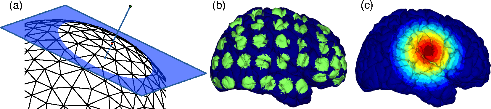

A region of the cortex was selected by identifying all mesh nodes that fall inside a sphere of variable radius centered on each of the 329 projected positions on the cortex, as illustrated in Fig. 4(b). The PSFs centered at each of the selected nodes were added for both EEG and NIRS. Then, a NIRS-EEG correlation value was calculated for each ROI from the correlation of the added PSFs. Then, the correlation values were assigned to all nodes within the ROI; the correlation values were averaged for nodes that belonged to multiple regions. This ROI analysis was repeated for varying spherical ROI radii, as shown in Fig. 4(c). The correlation values were averaged across all nodes for each ROI size, and the optimal ROI size was calculated as the one that yielded the maximum average correlation. Finally, a correlation value for each node was calculated using the ROI method and the optimal ROI radius.

3. Results

3.1.

NIRS-EEG Sensitivity Correlation

The correlations between each EEG electrode channel and NIRS source-detector pair calculated with Eq. (21) had a maximum value of $R_{max} = 0.28$ , as is shown in Fig. 5(a). All values of NIRS and EEG sensitivities below the $CNR = 0 dB$ threshold set were set to zero to ignore the noise when calculating the correlations. The new correlations using the thresholded NIRS sensitivity had a maximum value of $R_{max} = 0.58$ , as is shown in Fig. 5(b).

Fig. 5

(a) Correlation between NIRS source-detector pair sensitivities and EEG electrode sensitivities. (b) Correlation between (noise-thresholded) EEG electrode sensitivity and (noise-thresholded) NIRS source-detector pair sensitivity. [The NIRS and EEG sensitivities were set to zero for CNR values below 0 dB].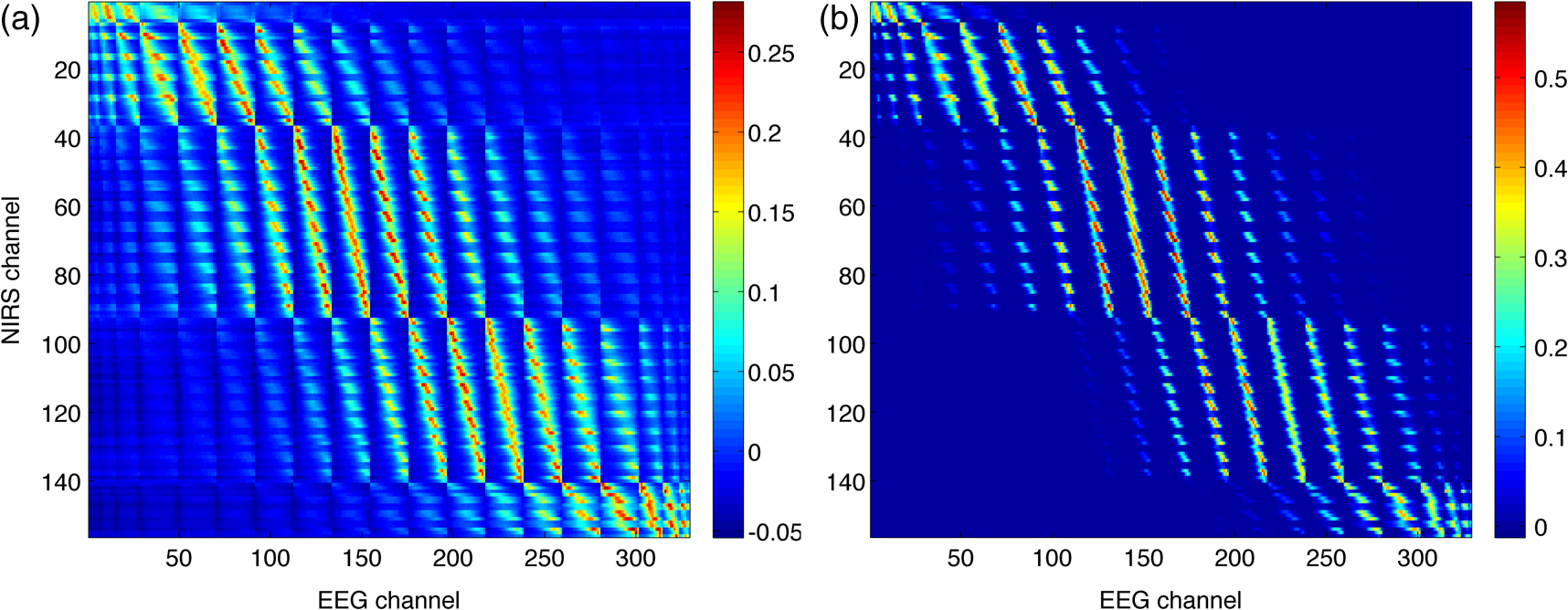

NIRS source-detector pair groups, based on the maximum sensitivity correlation to their corresponding EEG electrode, were calculated. The optimal groups were selected based on the channels with the highest correlations from Fig. 5(b) for each EEG channel. The correlation values between each EEG channel and optimal NIRS source-detector pair group have a mean and standard deviation of $R = 0.46 \pm 0.08$ across all 329 positions and are shown in Fig. 6. The correlation values are placed at each EEG electrode position.

Fig. 6

Correlation between optimal NIRS source-detector pair group sensitivity and EEG electrode sensitivity for each corresponding EEG channel with mean 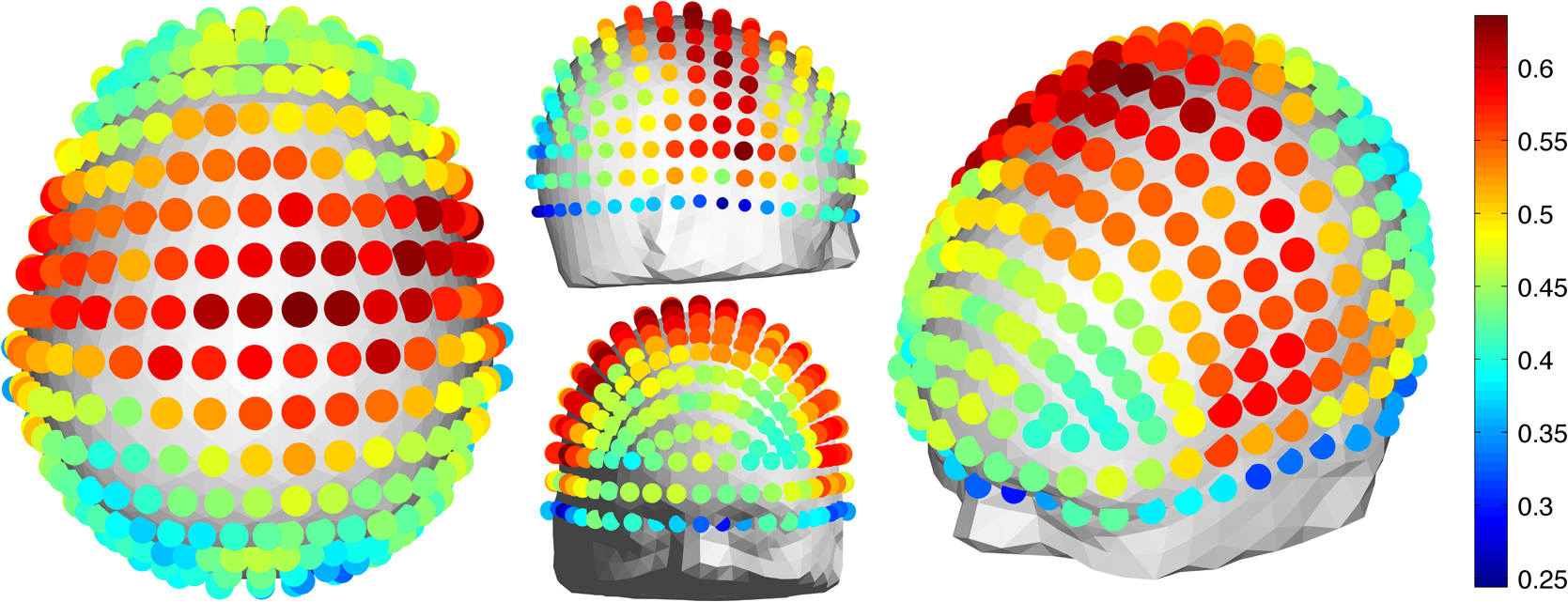$R = 0.46 \pm 0.08$ .

The reference table of source-detector pair groupings with respect to each electrode generated contains the optimal source-detector pair group that corresponds to each electrode. The table was calculated from the subset of 65 EEG electrode positions (EEG 10-10) that were chosen. The number $k$ of source-detector pairs required to obtain the maximum sensitivity correlation in each optimal group with respect to each EEG channel is shown in Fig. 7. Given that the top 50% of optimal groups required four pairs or less for maximum correlation with each EEG channel, the first four (or less) pairs for each group—sorted to be the ones with the highest correlation to that EEG channel—were were combined as individual effective NIRS channels. This threshold $(k = 4)$ is shown in the red dashed line in Fig. 7. The thresholded grouped pairs required for maximum correlation are listed in Table 2. For each electrode, Table 2 lists the first four optode source-detector pairs that will maximally correlate to it. The correlation between each EEG channel and its corresponding thresholded optimal NIRS source-detector pair group has a mean and standard deviation of $R = 0.44 \pm 0.08$ across all 65 positions selected. The position for each source-detector pair included in each group, the corresponding EEG electrode, and their labels are shown in Fig. 1.

Fig. 7

Histogram of optimal source-detector pair sensitivity groupings, displaying the amount of source-detector pairs required on each optimal group so that each group’s sensitivity achieves maximum correlation to the group’s corresponding EEG electrode. A subset of 65 electrodes was selected for this calculation based on the EEG 10-10 positioning layout. The red dashed line displays the threshold $(k = 4)$ for the optimal groups chosen.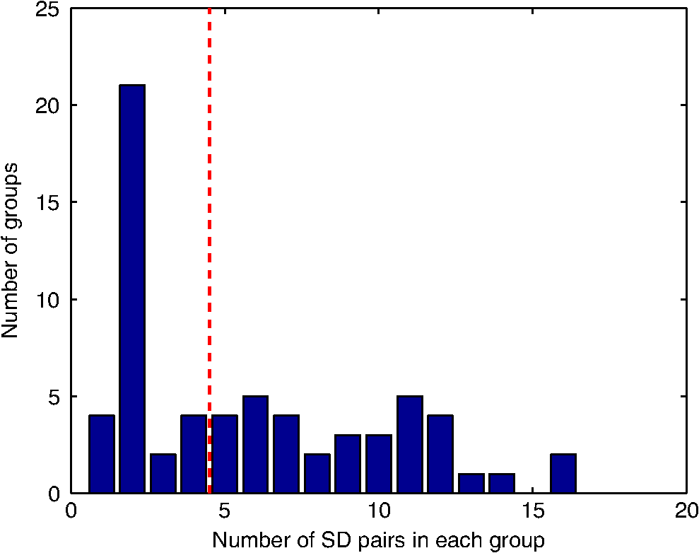

3.2.

NIRS-EEG Inverse Model Correlation

The correlation values at each node from the EEG and NIRS inverse models are shown in Fig. 8. The mean correlation between the PSFs for EEG and NIRS was $R = 0.17 \pm 0.10$ . Figure 8 illustrates the correspondence between EEG and NIRS tomographic sensitivities above the CNR threshold. The correlations between EEG and NIRS PSFs were computed for 329 spherical ROIs evenly distributed throughout the surface of the cortex with varying radii. Spherical ROIs with a radius of 26 mm yielded the maximum correlation between EEG and NIRS averaged across all cortical mesh nodes, as shown in Fig. 9. Using 329 ROIs with radii of 26 mm, the mean correlation between the PSFs for EEG and NIRS ROIs was $R = 0.43 \pm 0.07$ , as shown in Fig. 10. Figure 10 also illustrates the correspondence between EEG and NIRS tomographic sensitivities above the CNR threshold for measurements performed using 26 mm ROIs.

Fig. 8

Correlation between NIRS source-detector pair inverse model and EEG electrode inverse model for each brain mesh node with mean 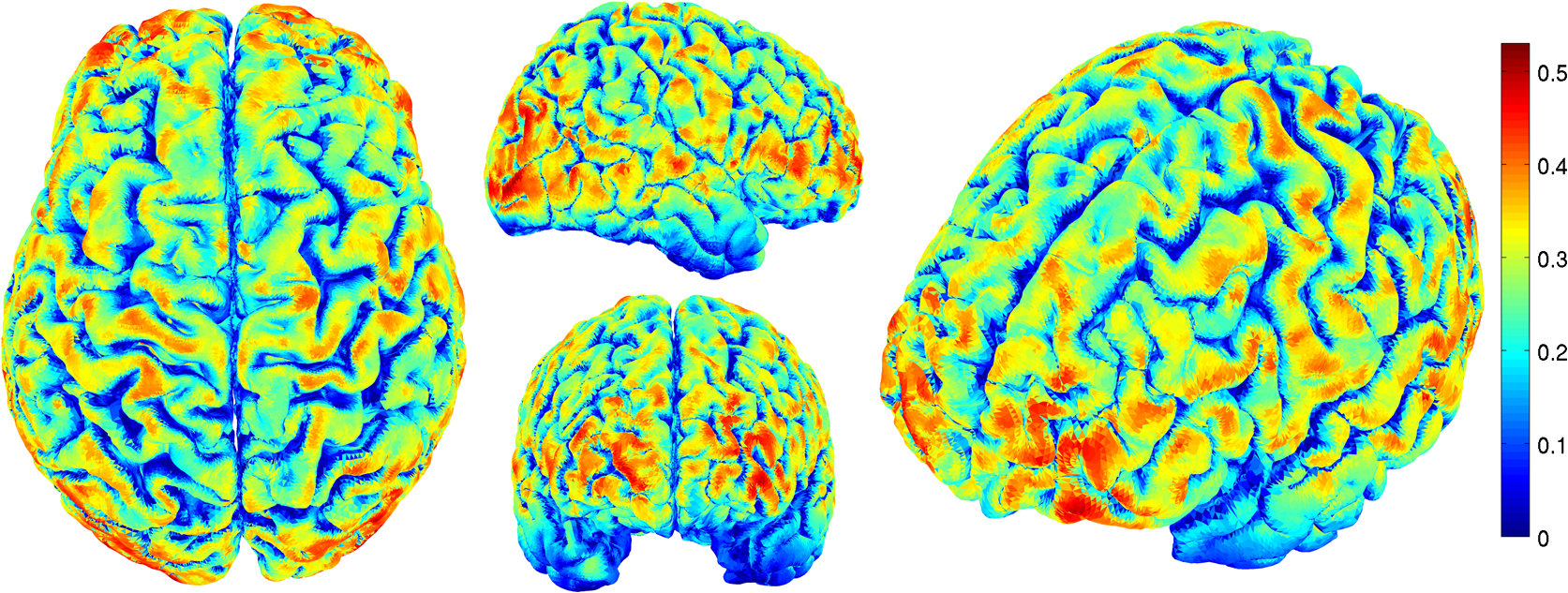$R = 0.17 \pm 0.10$ .

Fig. 9

Mean (bold line) and standard deviations (dashed lines) of the region of interest correlation between NIRS source-detector pair inverse model and EEG electrode inverse model for each ROI radius. The maximum mean correlation was obtained at a radius of 26 mm as marked with the vertical red line.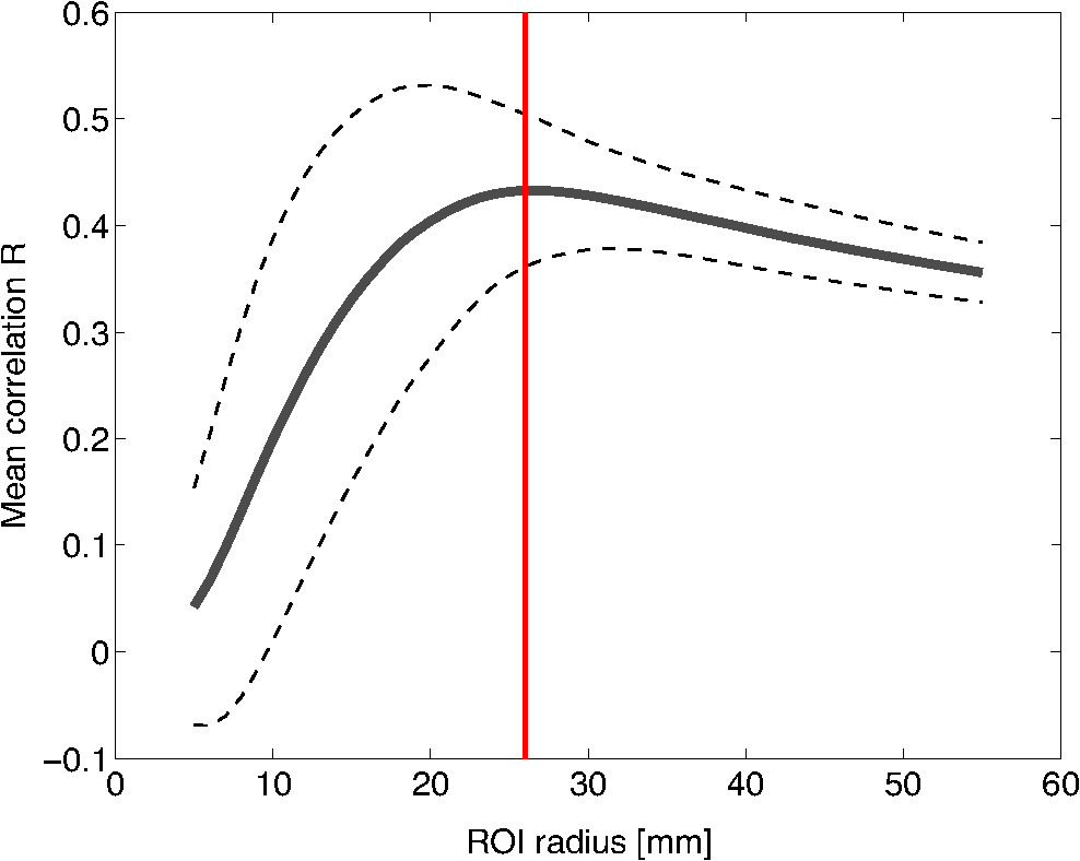

Fig. 10

ROI correlation between NIRS source-detector pair inverse model and EEG electrode inverse model for ROI radius of 26 mm with mean $R = 0.43 \pm 0.07$ .

4. Discussion

The sensitivity matrix of EEG and NIRS measurements to brain nodes illustrates the regions of the brain that are measured when using EEG or NIRS. Also, forward models can be combined to show sensitivity maps for the intersection of these two measurement types as applied in multimodal studies that combine EEG and NIRS to study the brain. Finally, the forward models provide the necessary data to compute inverse models for NIRS and EEG, yielding the tools needed to reconstruct tomographic maps of brain function. A principal use of the combination of EEG and NIRS in multimodal studies is to examine the relationship between neural signals and vascular hemodynamics as measured by EEG and NIRS, respectively. The interpretation of the data when using these systems depends on the location of the EEG electrodes and NIRS optodes and the intersection of the sensitivity to the brain from those locations. Meaningful conclusions regarding the neurovascular relationship can be drawn from NIRS and EEG data so long as the signals originate from the same region of the brain. In general, this can be assumed when using block studies to generate functional responses to a task that can be measured both with NIRS and EEG. But ultimately, these assumptions must be examined to understand the extent to which the origin of the EEG and NIRS signals spatially collocate. If the regions of the brain measured by the two systems do not intersect, then the interpretation regarding their relationship weakens. Neurovascular coupling studies that use NIRS and EEG will need to take into consideration the correlation between the sensitivities of the systems when interpreting the data, particularly when assuming that the recordings originate from the same brain regions. Likewise, the correspondence of the EEG and NIRS tomographic maps of the brain should be considered when drawing conclusions from the reconstructions of measurement data.

In order to understand the correspondence of the source of neural activity measured with EEG and hemodynamic responses simultaneously measured with NIRS, we studied the correlation of the sensitivity of NIRS and EEG to the brain using a layout that covers the whole head. The correlation values for each electrode and optimal source-detector pair group provide some insight into how multimodal data observe cortical activity, as illustrated in Fig. 6. The mean correlation of $R = 0.46 \pm 0.08$ obtained in this study suggests that the relationship between neural signals and vascular hemodynamics can only be studied to a limited extent with these systems and that revealing more precise relationships requires systems with sensitivities that correlate more strongly. Innovative experimental paradigms may need to be designed or analysis methods and modeling may need to be used to overcome this limitation.⁵¹^,⁵²

Also, the results (Fig. 6) show the spatial variation between the correlation of EEG and NIRS across different regions of the brain, suggesting that using EEG and NIRS for multimodal studies may be best suited to studies of certain cortical regions such as the primary sensorimotor areas. The causes of these regional differences could arise from a variety of factors including head and brain shapes, anatomical structure of head tissues, distance from the scalp to the brain, and the EEG–NIRS layout. Analysis of the relative contribution of these factors to the spatial variations in sensitivity correlation is beyond the scope of the present study. Given that NIRS and EEG sensitivities fall off with depth at different rates, the sensitivity of the intersection of EEG and NIRS is expected to be greatest near the surface. This can be seen in Fig. 8, where the nodal correlation is highest at the superficial regions of the gyri and lowest at the inner tissues within the sulci. The differences between the signal drop-off for EEG and NIRS can be seen in the example provided for the diagram in Fig. 3. The difference in sensitivity for each system possibly explains why a group of source-detector pairs is required—as opposed to a single pair—to correlate best to each electrode.

The spatial resolution of EEG and NIRS is the driving factor behind the ROI analysis results (Fig. 9). Computing correlations from individual nodal PSFs resulted in really low values (Fig. 8), suggesting that the analysis must be carried out using regions of activity as opposed to unitary sources. Computing correlations from larger regions yielded higher results and allowed the analysis of the size of those regions. Maximum average correlation across all nodes was obtained when running the analysis using a 26 mm radius ROI. This optimal ROI radius suggests that the interpretations regarding the correspondence between measurements carried out by EEG and NIRS may best be performed using regions of that size. The ROI analysis results highlight the need to consider the spatial extent of cortical activity when studying the multimodal data, a proposition consistent with studies that analyze sensitivity effects to spatial resolution of cortical activity.⁵³ Since NIRS measurements are performed between a source and detector pair, the source-detector separation approximates the spatial resolution of the measurements, usually several centimeters in length.⁵¹^,⁵⁴ EEG has similar spatial resolution to NIRS, on the order of centimeters, depending on the number of electrodes placed on the scalp, the orientation of the neurons, and the synchronicity of the signal.⁵⁵^,⁵⁶ The spatial resolution of these systems is comparable with the ROI correlation analysis results we obtained, where the maximum correlation is obtained for ROIs of a few centimeters.

The correlation between EEG and NIRS inverse models for the optimal ROI radius of 26 mm is shown in Fig. 10 and has a mean of $R = 0.43 \pm 0.07$ . This result agrees with the analysis performed on the correspondence of the sensitivity for NIRS and EEG (Fig. 6). The agreement between the sensitivity correlation analysis, carried out in electrode/optode space, and the ROI inverse model tomographic analysis, carried out in cortical space, was apparent in terms of the magnitude of correlation and its spatial distribution. For example, it can be seen from Figs. 6 and 10 that NIRS and EEG correspond maximally in the motor cortex. This agreement could indicate that selecting the optimal NIRS optode source-detector group for each EEG electrode can yield measurements that correspond to signals originating from a region with a radius of several centimeters. The consistency among NIRS-EEG forward model correlations and inverse model correlations also points out the potential spatial limitations of these systems to study neurovascular coupling.

Studies have found the sensitivity of NIRS to detect hemodynamic responses to visual stimulation to be 36.8% without noise filtering and 55.2% with noise filtering.⁵⁷ This sensitivity is consistent with the joint NIRS-EEG sensitivities found in our correlation analyses. Innovative algorithms to reduce the noise from the signal may be needed in studies to improve the sensitivity of NIRS and EEG to the brain and to improve the correlation between the signals recorded with these systems. Computing the joint forward model for NIRS and EEG and using the systems simultaneously may be useful beyond the studies of neurovascular coupling, as their corresponding sensitivities can be used as statistical priors to obtain more information from the signals with respect to their independent analysis, to improve their spatiotemporal resolution, or to reduce the number of electrodes or optodes required for measurement of a ROI.¹⁸ NIRS hemodynamic responses have been shown to be useful statistical priors for the estimation of cortical currents from EEG signals.¹⁸ The joint forward and inverse models studied in this work can be used in similar ways to investigate the source of brain activity when simultaneously, consecutively, and independently measured by NIRS and EEG.

The forward model analysis yielded optimal source-detector groups that correlate maximally with each electrode. The agreement between the results obtained in forward model analysis (Fig. 6) and the inverse model analysis (Fig. 10) suggests that the correlation values we obtained in the cortex can be expected by experimenters using the source-detector pairs and electrodes we utilized without requiring the computation of the NIRS and EEG forward or inverse model analyses. For that purpose, we generated an itemized list (Table 2) of NIRS source-detector pair groups that best correspond to each EEG electrode (for a subset of 65 electrodes that follow the EEG 10-10 layout). This list may be used by experimenters to select which electrodes and optodes simultaneously correspond to a cortical ROI. This information could be used for example by researchers to determine which electrodes and optodes to include when studying functional networks, by clinicians to select electrode and optode locations for chronic monitoring, or in the design of EEG and NIRS brain-computer interfaces where it is desirable to minimize the number of electrodes or optodes used. Also, Table 2 can be used by experimenters who have EEG electrodes and need to know which NIRS optodes will yield the best multimodal recordings or by those who have a specific region of the brain they are interested in studying and need to know where to place their electrodes and optodes to obtain the best results. It is worth noting that there is some expected variation in the correlation values obtained in this study when a different NIRS/EEG layout is used, when studying children, or when the electrical or optical coupling is not optimal, yielding a bad signal for certain channels.

Finally, the methods introduced in this study use the standard techniques from EEG electrode positioning and apply those same principles to NIRS in order to standardize NIRS channels, optode positioning, and the correspondence of optodes and cortical locations. The standardization of NIRS, particularly for EEG–NIRS studies, will aid in experiment-planning and interpretation of the signals. In addition, joint forward model and inverse model solutions as shown in this study provide the necessary data to perform tomographic imaging from multimodal studies combining EEG and NIRS.

Acknowledgments

This work was supported by the NIH National Institute of Aging R21AG033256, Dartmouth SYNERGY, and the Institute for Quantitative Biomedical Sciences (iQBS).

References

1.

T. MushaY. Okamoto, “Forward and inverse problems of EEG dipole localization,” Crit. Rev. Biomed. Eng., 27 (3–5), 189 –239 (1999). CRBEDR 0278-940X Google Scholar

2.

V. JurcakD. TsuzukiI. Dan, “10/20, 10/10, and 10/5 systems revisited: their validity as relative head-surface-based positioning systems,” NeuroImage, 34 (4), 1600 –1611 (2007). http://dx.doi.org/10.1016/j.neuroimage.2006.09.024 NEIMEF 1053-8119 Google Scholar

3.

V. L. Towleet al., “The spatial location of EEG electrodes: locating the best-fitting sphere relative to cortical anatomy,” Electroencephalogr. Clin. Neurophysiol., 86 (1), 1 –6 (1993). http://dx.doi.org/10.1016/0013-4694(93)90061-Y ECNEAZ 0013-4694 Google Scholar

4.

P. GiacomettiS. G. Diamond, “Diffuse optical tomography for brain imaging: continuous wave instrumentation and linear analysis methods,” Optical Methods and Instrumentation in Brain Imaging and Therapy, 57 –85 1st ed.Springer, New York (2013). Google Scholar

5.

C. Iadecola, “Neurovascular regulation in the normal brain and in Alzheimer’s disease,” Nat. Rev., 5 (5), 347 –360 (2004). http://dx.doi.org/10.1038/nrn1387 1474-175X Google Scholar

6.

H. GirouardC. Iadecola, “Neurovascular coupling in the normal brain and in hypertension, stroke, and Alzheimer disease,” J. Appl. Physiol., 100 (1), 328 –335 (2006). http://dx.doi.org/10.1152/japplphysiol.00966.2005 JAPYAA 0021-8987 Google Scholar

7.

B. V. Zlokovic, “The blood-brain barrier in health and chronic neurodegenerative disorders,” Neuron, 57 (2), 178 –201 (2008). http://dx.doi.org/10.1016/j.neuron.2008.01.003 NERNET 0896-6273 Google Scholar

8.

J. A. H. R. ClaassenR. Zhang, “Cerebral autoregulation in Alzheimer’s disease,” J. Cereb. Blood Flow Metab., 31 (7), 1572 –1577 (2011). http://dx.doi.org/10.1038/jcbfm.2011.69 JCBMDN 0271-678X Google Scholar

9.

B. Rosengartenet al., “Neurovascular coupling in Alzheimer patients: effect of acetylcholine-esterase inhibitors,” Neurobiol. Aging, 30 (12), 1918 –1923 (2009). http://dx.doi.org/10.1016/j.neurobiolaging.2008.02.017 NEAGDO 0197-4580 Google Scholar

10.

H. Laufs, “A personalized history of EEG-fMRI integration,” NeuroImage, 62 (2), 1056 –1067 (2012). http://dx.doi.org/10.1016/j.neuroimage.2012.01.039 NEIMEF 1053-8119 Google Scholar

11.

B.-M. Mackertet al., “Neurovascular coupling analyzed non-invasively in the human brain,” NeuroReport, 15 (1), 63 –66 (2004). http://dx.doi.org/10.1097/00001756-200401190-00013 NERPEZ 0959-4965 Google Scholar

12.

B. Heet al., “Electrophysiological imaging of brain activity and connectivity-challenges and opportunities,” IEEE Trans. Biomed. Eng., 58 (7), 1918 –1931 (2011). http://dx.doi.org/10.1109/TBME.2011.2139210 IEBEAX 0018-9294 Google Scholar

13.

H. Hallezet al., “Review on solving the forward problem in EEG source analysis,” J. Neuroeng. Rehabil., 4 (1), 46 (2007). http://dx.doi.org/10.1186/1743-0003-4-46 1743-0003 Google Scholar

14.

S. VallaghéM. Clerc, “A global sensitivity analysis of three- and four-layer EEG conductivity models,” IEEE Trans. Biomed. Eng., 56 (4), 988 –995 (2009). http://dx.doi.org/10.1109/TBME.2008.2009315 IEBEAX 0018-9294 Google Scholar

15.

N. G. GençerC. E. Acar, “Sensitivity of EEG and MEG measurements to tissue conductivity,” Phys. Med. Biol., 49 (5), 701 –717 (2004). http://dx.doi.org/10.1088/0031-9155/49/5/004 PHMBA7 0031-9155 Google Scholar

16.

K. L. PerdueQ. FangS. G. Diamond, “Quantitative assessment of diffuse optical tomography sensitivity to the cerebral cortex using a whole-head probe,” Phys. Med. Biol., 57 (10), 2857 –2872 (2012). http://dx.doi.org/10.1088/0031-9155/57/10/2857 PHMBA7 0031-9155 Google Scholar

17.

M. A. Yücelet al., “Calibrating the BOLD signal during a motor task using an extended fusion model incorporating DOT, BOLD and ASL data,” NeuroImage, 61 (4), 1268 –1276 (2012). http://dx.doi.org/10.1016/j.neuroimage.2012.04.036 NEIMEF 1053-8119 Google Scholar

18.

T. Aiharaet al., “Cortical current source estimation from electroencephalography in combination with near-infrared spectroscopy as a hierarchical prior,” NeuroImage, 59 (4), 4006 –4021 (2012). http://dx.doi.org/10.1016/j.neuroimage.2011.09.087 NEIMEF 1053-8119 Google Scholar

19.

J. C. MosherR. M. LeahyP. S. Lewis, “EEG and MEG: forward solutions for inverse methods,” IEEE Trans. Biomed. Eng., 46 (3), 245 –259 (1999). http://dx.doi.org/10.1109/10.748978 IEBEAX 0018-9294 Google Scholar

20.

G. Addeet al., “Symmetric BEM formulation for the M/EEG forward problem,” in Information Processing in Medical Imaging Lecture Notes in Computer Science, 524 –535 (2003). Google Scholar

21.

A. Gramfortet al., “Open MEEG: opensource software for quasistatic bioelectromagnetics,” Biomed. Eng. Online, 9 (45), 1 –20 (2010). http://dx.doi.org/10.1186/1475-925X-9-45 1475-925X Google Scholar

22.

J. Kybicet al., “A common formalism for the integral formulations of the forward EEG problem,” IEEE Trans. Med. Imaging, 24 (1), 12 –28 (2005). http://dx.doi.org/10.1109/TMI.2004.837363 ITMID4 0278-0062 Google Scholar

23.

J. GuanS. FangC. Guo, “Optical tomography reconstruction algorithm based on the radiative transfer equation considering refractive index-Part 1: forward model,” Comput. Med. Imaging Graph., 37 (3), 245 –255 (2013). http://dx.doi.org/10.1016/j.compmedimag.2013.01.005 CMIGEY 0895-6111 Google Scholar

24.

J. GuanS. FangC. Guo, “Optical tomography reconstruction algorithm based on the radiative transfer equation considering refractive index-Part 2: inverse model,” Comput. Med. Imaging Graph., 37 (3), 256 –262 (2013). http://dx.doi.org/10.1016/j.compmedimag.2013.01.006 CMIGEY 0895-6111 Google Scholar

25.

M. Hiraokaet al., “A Monte Carlo investigation of optical pathlength in inhomogeneous tissue and its application to near-infrared spectroscopy,” Phys. Med. Biol., 38 (12), 1859 –1876 (1993). http://dx.doi.org/10.1088/0031-9155/38/12/011 PHMBA7 0031-9155 Google Scholar

26.

L. KocsisP. HermanA. Eke, “The modified Beer-Lambert law revisited,” Phys. Med. Biol., 51 (5), N91 –N98 (2006). http://dx.doi.org/10.1088/0031-9155/51/5/N02 PHMBA7 0031-9155 Google Scholar

27.

E. OkadaD. T. Delpy, “Near-infrared light propagation in an adult head model. II. Effect of superficial tissue thickness on the sensitivity of the near-infrared spectroscopy signal,” Appl. Opt., 42 (16), 2915 –2922 (2003). http://dx.doi.org/10.1364/AO.42.002915 APOPAI 0003-6935 Google Scholar

28.

H. Dehghaniet al., “Near infrared optical tomography using NIRFAST: algorithm for numerical model and image reconstruction,” Commun. Numer. Methods Eng., 25 (6), 711 –732 (2008). http://dx.doi.org/10.1002/cnm.v25:6 CANMER 0748-8025 Google Scholar

29.

Y. Hoshi, “Functional near-infrared spectroscopy: potential and limitations in neuroimaging studies,” Int. Rev. Neurobiol., 66 237 –266 (2005). http://dx.doi.org/10.1016/S0074-7742(05)66008-4 IRNEAE 0074-7742 Google Scholar

30.

E. OkadaD. T. Delpy, “Near-infrared light propagation in an adult head model. I. Modeling of low-level scattering in the cerebrospinal fluid layer,” Appl. Opt., 42 (16), 2906 –2914 (2003). http://dx.doi.org/10.1364/AO.42.002906 APOPAI 0003-6935 Google Scholar

31.

E. Okadaet al., “Theoretical and experimental investigation of near-infrared light propagation in a model of the adult head,” Appl. Opt., 36 (1), 21 –31 (1997). http://dx.doi.org/10.1364/AO.36.000021 APOPAI 0003-6935 Google Scholar

32.

M. ClercJ. Kybic, “Cortical mapping by LaplaceCauchy transmission using a boundary element method,” Inverse Probl., 23 (6), 2589 –2601 (2007). http://dx.doi.org/10.1088/0266-5611/23/6/020 INPEEY 0266-5611 Google Scholar

33.

B. HeY. WangD. Wu, “Estimating cortical potentials from scalp EEG’s in a realistically shaped inhomogeneous head model by means of the boundary element method,” IEEE Trans. Biomed. Eng., 46 (10), 1264 –1268 (1999). http://dx.doi.org/10.1109/10.790505 IEBEAX 0018-9294 Google Scholar

34.

S. R. Arridge, “Optical tomography in medical imaging,” Inverse Probl., 15 (2), R41 –R93 (1999). http://dx.doi.org/10.1088/0266-5611/15/2/022 INPEEY 0266-5611 Google Scholar

35.

P. GiacomettiK. L. PerdueS. G. Diamond, “Algorithm to find high density EEG scalp coordinates and analysis of their correspondence to structural and functional regions of the brain,” J. Neurosci. Methods, 229 (C), 84 –96 (2014). http://dx.doi.org/10.1016/j.jneumeth.2014.04.020 JNMEDT 0165-0270 Google Scholar

36.

R. Vincent, “BrainWeb: simulated brain database,” (2012). http://www.bic.mni.mcgill.ca/brainweb/ Google Scholar

37.

B. Aubert-Brocheet al., “Twenty new digital brain phantoms for creation of validation image data bases,” IEEE Trans. Med. Imaging, 25 (11), 1410 –1416 (2006). http://dx.doi.org/10.1109/TMI.2006.883453 ITMID4 0278-0062 Google Scholar

38.

F. Tadelet al., “Brainstorm: a user-friendly application for MEG/EEG analysis,” Comput. Intell. Neurosci., 2011 879716 (2011). http://dx.doi.org/10.1155/2011/879716 Google Scholar

39.

B. FischlM. I. SerenoA. M. Dale, “Cortical surface-based analysis. II: inflation, flattening, and a surface-based coordinate system,” NeuroImage, 9 (2), 195 –207 (1999). http://dx.doi.org/10.1006/nimg.1998.0396 NEIMEF 1053-8119 Google Scholar

40.

A. M. DaleB. FischlM. I. Sereno, “Cortical surface-based analysis. I. Segmentation and surface reconstruction,” NeuroImage, 9 (2), 179 –194 (1999). http://dx.doi.org/10.1006/nimg.1998.0395 NEIMEF 1053-8119 Google Scholar

41.

B. Fischl, “FreeSurfer,” NeuroImage, 62 (2), 774 –781 (2012). http://dx.doi.org/10.1016/j.neuroimage.2012.01.021 NEIMEF 1053-8119 Google Scholar

42.

M. Reuteret al., “Within-subject template estimation for unbiased longitudinal image analysis,” NeuroImage, 61 (4), 1402 –1418 (2012). http://dx.doi.org/10.1016/j.neuroimage.2012.02.084 NEIMEF 1053-8119 Google Scholar

43.

S. MurakamiY. Okada, “Contributions of principal neocortical neurons to magnetoencephalography and electroencephalography signals,” J. Physiol., 575 (3), 925 –936 (2006). http://dx.doi.org/10.1113/jphysiol.2006.105379 JPHYA7 0022-3751 Google Scholar

44.

M. Hämäläinenet al., “Magnetoencephalographytheory, instrumentation, and applications to noninvasive studies of the working human brain,” Rev. Mod. Phys., 65 (2), 413 –497 (1993). http://dx.doi.org/10.1103/RevModPhys.65.413 RMPHAT 0034-6861 Google Scholar

45.

M. S. HämäläinenR. J. Ilmoniemi, “Interpreting magnetic fields of the brain: minimum norm estimates,” Med. Biol. Eng. Comput., 32 (1), 35 –42 (1994). http://dx.doi.org/10.1007/BF02512476 MBECDY 0140-0118 Google Scholar

46.

Q. Fang, “Mesh-based Monte Carlo method using fast ray-tracing in Plücker coordinates,” Biomed. Opt. Express, 1 (1), 165 –175 (2010). http://dx.doi.org/10.1364/BOE.1.000165 BOEICL 2156-7085 Google Scholar

47.

Q. FangD. A. Boas, “Tetrahedral mesh generation from volumetric binary and grayscale images,” in Proc. of IEEE International Symp. on Biomedical Imaging (ISBI 2009), 1142 –1145 (2009). Google Scholar

48.

Y. Zhanet al., “Image quality analysis of high-density diffuse optical tomography incorporating a subject-specific head model,” Front. Neuroenerg., 4 (May), 6 (2012). http://dx.doi.org/10.3389/fnene.2012.00006 FNREJG 1662-6427 Google Scholar

49.

A. H. Bamettet al., “Robust inference of baseline optical properties of the human head with three-dimensional segmentation from magnetic resonance imaging,” Appl. Opt., 42 (16), 3095 –3108 (2003). http://dx.doi.org/10.1364/AO.42.003095 APOPAI 0003-6935 Google Scholar

50.

P. GiacomettiS. G. Diamond, “Compliant head probe for positioning electroencephalography electrodes and near-infrared spectroscopy optodes,” J. Biomed. Opt., 18 (2), 027005 (2013). http://dx.doi.org/10.1117/1.JBO.18.2.027005 JBOPFO 1083-3668 Google Scholar

51.

D. K. Josephet al., “Diffuse optical tomography system to image brain activation with improved spatial resolution and validation with functional magnetic resonance imaging,” Appl. Opt., 45 (31), 8142 –8151 (2006). http://dx.doi.org/10.1364/AO.45.008142 APOPAI 0003-6935 Google Scholar

52.

S. G. Diamondet al., “Dynamic physiological modeling for functional diffuse optical tomography,” NeuroImage, 30 (1), 88 –101 (2006). http://dx.doi.org/10.1016/j.neuroimage.2005.09.016 NEIMEF 1053-8119 Google Scholar

53.

K. L. PerdueS. G. Diamond, “Effects of spatial pattern scale of brain activity on the sensitivity of DOT, fMRI, EEG and MEG,” PloS One, 8 (12), e83299 (2013). http://dx.doi.org/10.1371/journal.pone.0083299 1932-6203 Google Scholar

54.

D. A. Boaset al., “Improving the diffuse optical imaging spatial resolution of the cerebral hemodynamic response to brain activation in humans,” Opt. Lett., 29 (13), 1506 –1508 (2004). http://dx.doi.org/10.1364/OL.29.001506 OPLEDP 0146-9592 Google Scholar

55.

T. FerreeM. ClayD. Tucker, “The spatial resolution of scalp EEG,” Neurocomputing, 38–40 1209 –1216 (2001). http://dx.doi.org/10.1016/S0925-2312(01)00568-9 NRCGEO 0925-2312 Google Scholar

56.

H. Shibasaki, “Human brain mapping: hemodynamic response and electrophysiology,” Clin. Neurophysiol., 119 (4), 731 –743 (2008). http://dx.doi.org/10.1016/j.clinph.2007.10.026 CNEUFU 1388-2457 Google Scholar

57.

M. Biallaset al., “Reproducibility and sensitivity of detecting brain activity by simultaneous electroencephalography and near-infrared spectroscopy,” Exp. Brain Res., 222 (3), 255 –264 (2012). http://dx.doi.org/10.1007/s00221-012-3213-6 EXBRAP 0014-4819 Google Scholar

Biography

Paolo Giacometti received a Bachelor of Arts degree in applied physics with a minor in computational physical science from Saint Anselm College in 2009 and a PhD in engineering sciences from Dartmouth College in 2014. His doctoral dissertation focused on multimodal electroencephalography and near-infrared spectroscopy neuroimaging measurement and analysis. He is currently conducting postdoctoral training at the Multimodal Neuroimaging Lab at the Thayer School of Engineering at Dartmouth.

Solomon Diamond received an AB degree in engineering sciences from Dartmouth College in 1997, a BE degree from the Thayer School of Engineering at Dartmouth in 1998, and a PhD in engineering sciences from Harvard University in 2004. He conducted postdoctoral training at the Martinos Center for Biomedical Imaging at Massachusetts General Hospital. He is currently an associate professor at Dartmouth where he teaches courses in machine design, computer-aided design, and neuroengineering.

Citation Download Citation

Paolo Giacometti and Solomon G. Diamond "Correspondence of electroencephalography and near-infrared spectroscopy sensitivities to the cerebral cortex using a high-density layout," Neurophotonics 1(2), 025001 (2 September 2014). https://doi.org/10.1117/1.NPh.1.2.025001

Published: 2 September 2014

Access the abstract

JOURNAL ARTICLE
14 PAGES

DOWNLOAD PAPER SAVE TO MY LIBRARY

GET CITATION

CITATIONS

Cited by 14 scholarly publications.

Explore citations on Lens.org

RIGHTS & PERMISSIONS

Get copyright permission Get copyright permission on Copyright Marketplace

KEYWORDS

Electroencephalography

Near infrared spectroscopy

Electrodes

Brain

Sensors

Head

Point spread functions

1.

Introduction

1.1.

EEG Forward Model

Eq. (1)

1.2.

NIRS Forward Model

Eq. (2)

Eq. (3)

Eq. (4)

Eq. (5)

1.3.

EEG and NIRS Inverse Models

2.

Methods

2.1.

EEG Forward Model

Eq. (6)

2.2.

EEG Inverse Model

Eq. (7)

Eq. (8)

2.3.

NIRS Forward Model

Eq. (9)

Fig. 1

Table 1

Fig. 2

Eq. (10)

Eq. (11)

Eq. (12)

Eq. (13)

Eq. (14)

Eq. (15)

Eq. (16)

Eq. (17)

Eq. (18)

2.4.

NIRS Inverse Model

Eq. (19)

Eq. (20)

2.5.

NIRS–EEG Sensitivity Correlation

Eq. (21)

Table 2

2.6.

NIRS-EEG Inverse Model Correlation

Eq. (22)

Fig. 3

Fig. 4

3.

Results

3.1.

NIRS-EEG Sensitivity Correlation

Fig. 5

Fig. 6

Fig. 7

3.2.

NIRS-EEG Inverse Model Correlation

Fig. 8

Fig. 9

Fig. 10

4.

Discussion

Acknowledgments

References

Biography

Show All Keywords

Keywords/Phrases

Search In:

Publication Years