|
|
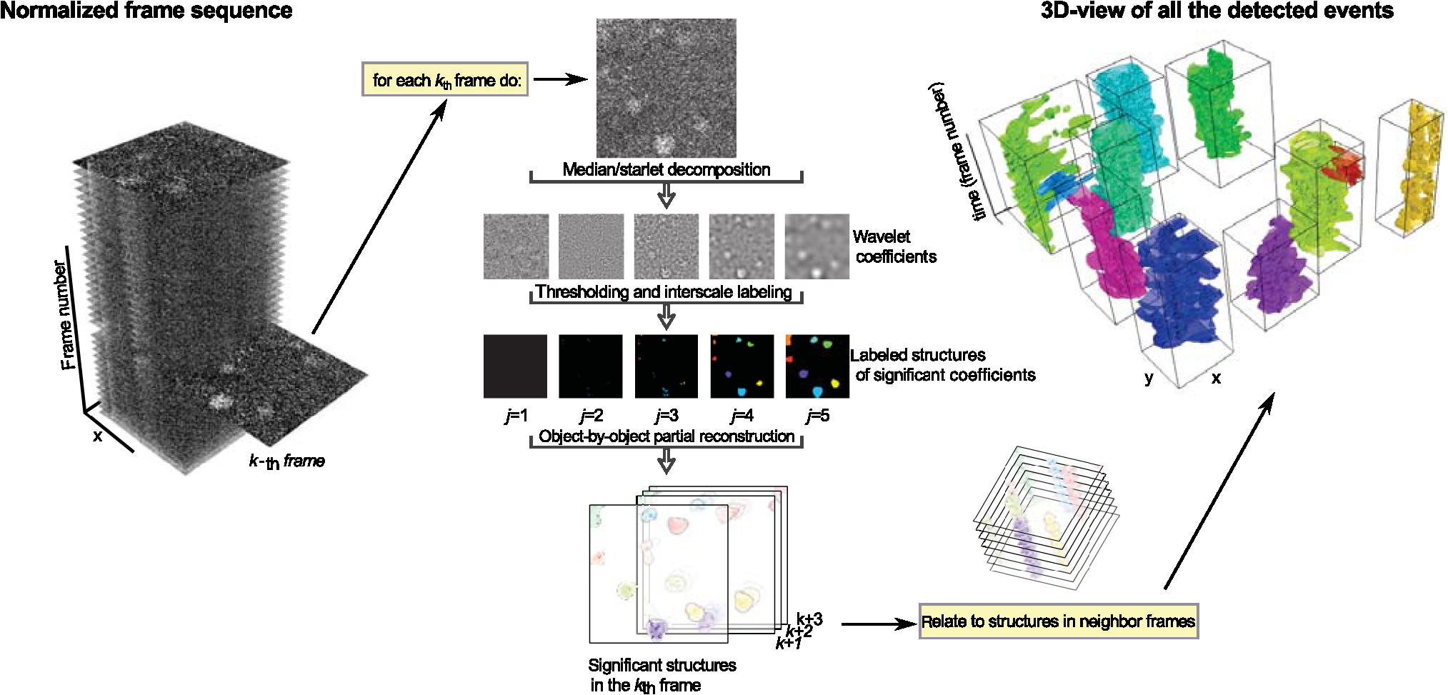
1.IntroductionModern imaging techniques, including two-photon microscopy, produce in vivo experimental data of great diversity and volume. New experimental possibilities, such as optogenetics, bring about new scientific questions to address and consequently generate a torrent of data. One of the existing problems is the compromise between a demand for fast sampling to resolve rapid transient processes on one hand and sufficient spatial resolution on the other hand. Although imaging data tend to be collected in high detail, a large portion of it contains background or noise and is discarded downstream in the processing pipeline, while a small fraction is considered the useful “signal.” It is important to robustly identify the useful parts of data in low signal-to-noise ratio (SNR) measurements. An important feature of analyzed data is its sparseness or compressibility under some transform, i.e., if the data can be decomposed into some basis such as Fourier or wavelet, where only a few coefficients are significantly larger than zero. The notion of sparseness is essential for noise suppression. If transformed data are sparse, one can legitimately assume that only the few large coefficients contain information about the underlying signal, whereas the small-valued coefficients can be attributed to noise. This leads to the idea of thresholding in a transform space for image enhancement.1,2 Because wavelet transform provides a nearly sparse representation of piecewise smooth images,3 this transform and its variants have become popular in image denoising and signal detection in transform domain,4–8 although there are also other transforms that can provide sparse representation, such as singular value decomposition and Radon transform. In short, wavelet transform is a multiscale representation of the input data, obtained via iterative application of band-pass filters. Wavelet coefficients capture the signal features at different locations and hierarchical spatial resolutions. The multiscale property is particularly useful for denoising because a typical useful signal is sparse (concentrated in a few coefficients at several scales), while noise is homogeneously distributed. Calcium signaling in astrocytes takes versatile forms, one of which is spatially patterned spreading signals that pervade astroglial networks. Intercellular waves in astrocytic syncytium can be triggered by electrical and mechanical stimulations,9 local elevation of extracellular adenosine triphosphate (ATP) level,10 or by neuronal activity in situ11 Spontaneous glial calcium signaling is reported to guide axonal growth and cell migration in the developing brain,12–14 and calcium waves may represent a reaction to local tissue damage or other pathology. For instance, the incidence of spontaneous waves is increased with aging and low-oxygen conditions.15 Detection and reconstruction of waves in fluorescent imaging recordings pose challenges for data analysis. The key problem is identifying transient low contrast events in large series of images at a low SNR. Conventional data analysis methods can be loosely categorized to region of interest (ROI) type analyses, pixel thresholding, statistical component analyses, and multiscale (usually wavelet based) analyses. ROI analysis and pixel thresholding work particularly well with evoked responses, easily recognizable cellular correlates, relatively low noise, and small datasets. An ROI-based approach is primarily popular because it is often simple to select the ROIs corresponding to neuronal bodies and then process the ROI-averaged fluorescence traces. However, it becomes unwieldy for the analysis of sparse spontaneous events in large datasets and high noise levels or where a priori selection of regions of interest is impossible, which is the case for waves in the molecular layer of the cerebellum. Independent component analysis (ICA)16 is capable of processing large datasets with sparse spontaneous events, but has some limitations. Specifically, the output of ICA relies on the independence of the analyzed signals, and does not preserve the relative amplitude or sign of the detected components; in application to frame series it does not directly take advantage of local correlations in pixel intensities. Spontaneously occurring glial waves (GCWs) are hard to detect and quantify by ROI analysis, pixel thresholding, or ICA. In this paper, we present an example of a multiscale approach to image and signal processing. We discuss a framework for the multiscale vision model (MVM)17,18 in application to the problem of detection and reconstruction of spontaneous intercellular glial waves. This technique relies on the sparsifying property of the wavelet transform. In short, wavelet transform is a multiscale representation of the input data, made via iterative application of band-pass filters. Wavelet coefficients capture the signal features at different locations and hierarchical spatial resolutions. Due to the nature of the used transform, MVM is most suitable for detection of nearly round faint structures in noisy images or bright blobs in three-dimensional (3-D) data. Because glial calcium waves are manifested as expanding nearly isotropic transient fluorescent elevations, MVM performs well in pursuing such structures frame after frame, and then stitching overlapping objects as snapshots of a single GCW event. 2.Multiscale Vision Model for Detection of Glial Calcium WavesRecently, we adapted a wavelet-based framework, multiscale vision model to detect and analyze the spontaneous intercellular calcium waves in mouse cerebellum glial cells in vivo.18 In short, this framework amounts to noise rejection by thresholding wavelet coefficients of the input image, followed by establishing an interscale relationship between significant coefficients at different scales of decomposition and partial iterative reconstruction of the detected objects. Originally, this framework was suggested for the analysis of astronomy images19 and employed redundant wavelet transform with B-spline basis, also called “starlet” transform.2 Here, we report two improvements to our previous MVM implementation:18 (1) we increase the tolerance to outlier samples by using a mixed multiscale median and the starlet transform, and (2) we implement an iterative partial reconstruction algorithm. To illustrate this improved framework, we use several phantom patterns [Fig. 1(a)] of different shapes, contaminated with additive Gaussian white noise (AGWN) with a few bright “hot-spot” pixels with the noise variance in 0.05% of pixels [Fig. 1(b)]. This can also be described as a small amount of “salt noise” (SN). The framework is summarized in Fig. 4 using an experimental 2-pm record with a spontaneous glial wave in the mouse cerebellum as an example. The MVM framework is compared to other denoising techniques in Fig. 6 for phantoms and in Fig. 7 for the experimental recording. Fig. 1Test phantom patterns and their decompositions. (a) Pure patterns, patterns corrupted with additive Gaussian white noise (+AGWN), patterns corrupted with additive Gaussian white noise and salt noise (+AGWN+SN), (b) wavelet coefficients after the five-level starlet transform for the noisy patterns (+AGWN+SN), (c) coefficients of the multiscale median transform of the same pattern, (d) coefficients of the mixed multiscale median/starlet transform of the same pattern. 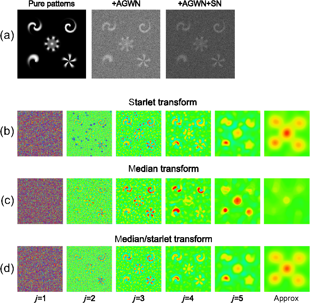 2.1.Starlet and Multiscale Median TransformsStarlet transfrom (also known as à trous transform) decomposes an original image into a set representing two-dimensional (2-D) image details at different scales (wavelet coefficients) and a smoothed approximation at the largest scale: where is the level of decomposition corresponding to a hierarchy of spatial scales. As increases, the coefficient images represent more and more coarse features of the original image . The starlet decomposition of a noisy phantom image is illustrated in Fig. 1. Wavelet coefficients at consecutive levels are iteratively obtained. First, the original image is considered an approximation at level 0 . Then, smoothed approximations at the level are obtained by convolution of the approximation at the level with a low-pass filter: and the wavelet coefficients (“details”) are defined as the difference between the subsequent approximations:The low-pass filter is zero-upsampled at each level, leading to interlaced image convolution. In the starlet transform, a discrete filter based on a cubic -spline is used. In one dimension (1-D), this filter takes the form . For 2-D images, one can use the outer product of the two one-dimensional filters or process each dimension separately with a 1-D filter. A known drawback of the starlet transform is that a very bright point structure will have responses in many scales instead of just being captured by the finest scale.2 Such small bright structures can be outliers, like occasional “hot pixels” of the charge coupled device matrix or salt noise. This is illustrated in the starlet decomposition of the phantom image, mixed with AGWN and salt noise [Fig. 1(b)], where the bright outlier points influence coefficients up to the fourth level of decomposition. Such a problem does not exist in the multiscale median transform [Fig. 1(c)]. This transform is organized in the same iterative way as the starlet transform, but the role of low-pass filtering is played by the median filter, with the window size doubling at each level of decomposition. In 2-Ds, the median filter of an image with window size can be defined as , i.e., each pixel in the image is replaced by the sample median of pixel values in the neigborhood of the pixel . The window size changes with the decomposition level as . The median filter is nonlinear and provides for robust smoothing, i.e., it attenuates the effect of outlier samples.2 Hence, one of the advantages of the multiscale median transform is better separation of structures in the scales, but the starlet transform provides a more robust noise estimation at different scales. In a compromise, one can mix the two transforms and use the median or starlet transform depending on the amplitude of the coefficient. In the original merged median/starlet transform (MST)2 at level , one first computes the median filtering of the approximation with a window size : Next, the temporary median transform coefficients are obtained, as . Then the high-intensity coefficients are defined as coefficients where , where MAD stands for the median absolute deviation and is used as a robust estimator of noise standard deviation, and threshold is chosen high enough to avoid false detections, usually . All the high-intensity coefficients in are set to zero and a version of with zeroed high-intensity structures is formed: . Next, the starlet transform of is done at scales (1), and the last approximation is finally used as . Thus, has been smoothed with wavelets after all strong features have been removed by median filtering. Because median filtering is computationally intensive and the outlying structures are usually small and thus are most frequent at small scales, we simplified the original algorithm by only performing the mixed decomposition at the first two scales and then continuing with the usual starlet transform. Coefficients of such a decomposition for the phantom image are shown in Fig. 1(d)—here all the hot-spot pixels are confined to the smallest scale coefficients and the structure of the patterns is more well preserved. Another example is shown in Fig. 2 for a noisy 1-D signal, which contains a Gaussian with at and an outlier sample with an amplitude the noise standard deviation at . Representation of the Gaussian object in the starlet coefficients at scale is affected by this sample, while the multiscale median and median/starlet transforms are free from this spurious influence and represent only the object of interest.Fig. 2Illustration of the influence of outlying samples on detection of objects in one-dimensional (1-D) signals. From top to bottom: analyzed signal, containing white noise, a Gaussian with at and an outlier with amplitude higher than the noise standard deviation at ; starlet coefficients at fifth level of decomposition; multiscale median transform coefficients at fifth level of decomposition; mixed median/starlet transform coefficients at fifth level of decomposition. The outlier distorts object of interest representation for starlet transform, but has no effect on multiscale median and mixed transforms. 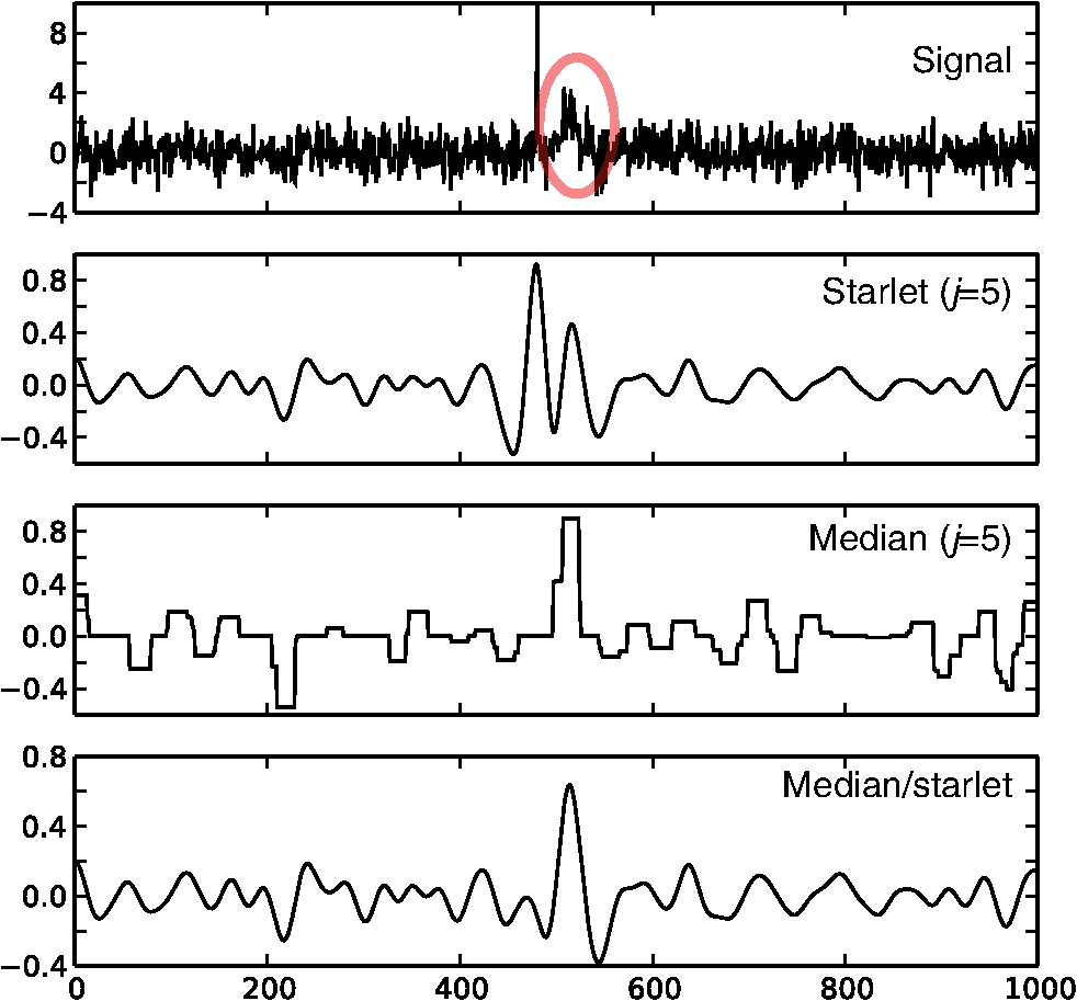 2.2.Significant Wavelet CoefficientsDetection of structures of interest that are significantly brighter than the background should be based on the knowledge about the statistical distribution of the wavelet coefficients in the background. We assumed stationary Gaussian white noise to set significance levels. Statistics of wavelet coefficients at each level were estimated with Monte Carlo simulations: we obtained standard deviations of noise wavelet coefficients at each level of decomposition (index 1 in represents unit variance). The obtained values were used as weighting factors for arbitrary noise variance in the analyzed images. More details can be found in Ref. 17 and in Chapter 2 of Ref. 20 The knowledge of noise standard deviations at different spatial scales allows the definition of significant coefficients for an image by thresholding at at each level. If , the coefficient is considered significant and possibly belonging to a bright object. Interested in elevations of , we only test positive coefficients corresponding to the luminous sources. The choice of can be varied for optimal performance; in the figures below, we used which corresponds to the 99.95th percentile of a Gaussian distribution. 2.3.Interscale Relationship and Object ReconstructionImage can be modeled as a composition of objects , smooth background , and noise : To recover the objects in a given image, we use contiguous regions of significant coefficients at each scale and establish their interscale connectivity relationships. Let a structure be a set of connected significant wavelet coefficients at scale : where are the coordinates of the ’th coefficient included in the structure. An example of such structures is given in Fig. 3(a), where the positions of significant median/starlet coefficients from Fig. 1(d) are shown in red. An object can be defined via a set of structures at several different levels: and the real object can be reconstructed from its wavelet representation . Structures in this set are hierarchically connected. Two structures at successive levels and are connected if the position of the maximum of wavelet coefficients belonging to the structure is also contained in . Some significant structures can also result from the noise. These structures are typically isolated, i.e., they are not connected to any structure at a lower or higher level. Such structures are discarded in the algorithm. Indeed, any structure can only be connected to one structure at the higher level and to more than one structure at the lower level, thus resulting in a branched tree-like connectivity graph. Such connectivity trees are illustrated in Fig. 3(b), where each tree is shown in a different color, and coefficients at different scales are overlaid. We can refer to these connectivity trees by their root nodes, i.e., the structures at the largest scale.Fig. 3Iterative reconstruction of the detected structures. (a) Masks for significant (shown in red) starlet/wavelet coefficients for the noisy image shown in Fig. 1, (b) labeled interscale trees of the significant starlet/wavelet coefficients, (c) norm of difference between the significant coefficients and decomposition of the reconstructed image for decomposition and reconstruction using the starlet transform (black circles), decomposition and reconstruction using the combined median/starlet transform (MST, blue diamonds), and decomposition using MST and reconstruction using the starlet transform (green triangles), (d) noisy image (+AGWN+SN), reconstructions using the different reconstruction variants shown in (c) and the residuals after subtracting the reconstructed image from the input image.  When there are several close objects or a smaller object is overlaid on a bigger one, the objects can become entangled in one connectivity tree and should be deblended. A structure will be detached from the tree as a new root node if there exists at least one other structure at the same level belonging to the same tree and the following condition is fulfilled: . Here, is the maximum wavelet coefficient of ; , where is the structure connected to , such that the position of its maximum wavelet coefficient is closest to the position of the maximum of , if is not connected to any structure at scale then ; and , i.e., the maximum wavelet coefficient at scale , such that its location belongs to . Recursive application of this deblending procedure to the connectivity tree yields objects as independent structures of significant wavelet coefficients. Partial reconstruction of these objects as images is a nontrivial task. The simplest solution is to perform inverse wavelet transforms for each object, setting all wavelet coefficients not belonging to the object to zero. In our previos study,18 we looked for a compromise between the computational speed and accuracy of reconstruction. For the sake of computational speed, we reconstructed objects simply as the inverse transform of the wavelet coefficients representing the object. Here, we improve our framework with an iterative reconstruction scheme.2 The idea is that we search for an image that will, under the multiscale transform (e.g., starlet), result in coefficients as close as possible to those to . Thus, we want to minimize by varying reconstruction image , where is the wavelet transform operator, and is the multiresolution support of , i.e., has ones where is nonzero and has zeros otherwise. The solution is searched iteratively: where is the inverse transform operator, , and step size can be damped at each iteration to ensure the stability of the solution. Reconstruction convergence can be seen from the decay of with the iteration number in Fig. 3(c) for the starlet transform (black points) and the median/starlet transform (blue diamonds). It is implied that the transform operator used for reconstruction in Eq. (7) is the same as the one used to obtain and , but this is not necessary. Noting that the median/starlet transform is computationally slower than the starlet transform and must be done multiple times in the iterative reconstruction algorithm, we tried to use the starlet transform as the in Eq. (7) (reconstruction operator is the same for these transforms). This trick is justified by the notion that it is unlikely that the starting image for reconstruction should contain any salt noise or outlier point structures, as the latter should have been rejected at the MST decomposition stage. This scheme led to surprisingly good results, shown in Fig. 3(c) (green triangles): the convergence is faster and better than in the starlet–starlet decomposition/reconstruction pair, and the reconstruction process is much less computationally intensive than in the MST-MST decomposition/reconstruction pair.The reconstruction results for the three decomposition/reconstruction pairs are shown in Fig. 3(d). We should note that in the reconstruction images, each of the pattern was independently reconstructed, but all the individual object reconstructions are summed in one image for the clarity of representation. The starlet-starlet variant retains the point structures along with the patterns, while the schemes involving the median/starlet transform reject this type of noise. Although the MST-MST scheme enhances the object contrast, the residual image (input minus the reconstruction) shows that it does not preserve initial object intensity, while the residual image for the MST-starlet scheme almost exclusively contains noise and little if any traces of the original patterns. This, together with a lower computational load, suggests the MST-starlet decomposition/reconstruction pair as the scheme of choice for the task of glial waves detection and reconstruction. The full MVM framework with the mixed median/starlet decomposition and iterative reconstruction to detect and recover spontaneous glial calcium waves is summarized in Fig. 4. For each frame of normalized imaging data, we perform the median/starlet decomposition and after thresholding find contiguous areas of significant coefficients. These structrures are linked into interscale tree-like connectivity trees (connected structures belonging to one object are shown in the same color in the figure). Based on these connectivity trees, iterative reconstruction using the starlet transform is individually done for each tree according to Eq. (7) (shown in different colors as “significant structures in the frame” in the figure). After this the procedure is done for all frames, and the individual objects contained in each frame are stored. The overlapping objects in the neighboring frames are linked into an 3-D representation of an evolution of distinct signaling events, shown as 3-D colored blobs in the scheme. Clearly, not all signaling events are glial waves, but after detection and 3-D reconstruction stages, one can identify the events of different types manually or according to any automated sorting scheme. 2.4.Comparison to Other Denoising TechniquesWe compared the MVM framework with our modifications to other modern denoising techniques, although an exhaustive survey of different denoising and object detection techniques is beyond the scope of this study. Figure 5(a) presents how the PSNR of denoised images changes with the PSNR of noise-corrupted images. Here, we compare the MVM, two algorithms of total variation (TV) denoising, which searches for image approximation with a minimal TV (integral of absolute gradient) and a bilateral filter.21 The TV denoising was used in two variants: the Chambolle algorithm22 and the split-Bregman algorithm.23 The TV and bilateral filtering implementations were used from the open-sourse scikit-image python library.24 Because the maximum value of the pure phantom image was 1, the PSNR was calculated as , where MSE is the mean square error between the tested image and the pure phantom image , each of size : . It is clear that with AGWN, the MVM resulted in a better PSNR of the recovered images at very low SNRs of the input images and had a similar performance [Fig. 5(a), left pane] to the TV/Chambolle algorithm at a higher PSNR of the input images, although MVM displayed much a higher performance scatter than the other algorithms at the higher PSNR of the input images. The better performance of the MVM at a very low PNSR of the noisy images likely results from background rejection in the MVM and exclusive reconstruction of only the detected structures. The addition of small amounts of salt noise (outlier pixels) did not affect the MVM performance, but deteriorated the performances of the other algorithms [Fig. 5(a), right pane]. It is clear that while the used denoising algorithms are not optimized for outlier measurements, preprocessing of the input images with filters, devoted for removal of salt noise, e.g., adaptive median filter, would have reverted the results to the case of a simple AGWN. Figure 5(b) visualizes the difference between denoising provided by the TV/Chambolle and the MVM approaches at different PSNR values for the degraded phantom image. Comparsion of the images denoised by the two algorithms supports the observation that the higher PSNR values achieved by MVM are due to setting the background to zero. Fig. 5Performance of the MVM and other state-of-the-art denoising techniques at different PSNR levels of the degraded phantom image shown in Fig. 1(a). (a) Resulting PSNR for images, denoised with the MVM (green) two total variation (TV) techniques with Chambolle (blue) and Bregman (yellow) algorithms, and a bilateral filter algorithm (pink) as a function of PSNR of input (degraded) images; input images are mixed with AGWN (left pane) or AGWN+SN (right pane). Shaded areas around the curves are between 0.05 and 0.95 quantiles of the observed PNSR values and continuous lines are median values (measured after 200 runs), (b) visual comparison between the TV/Chambolle and the MVM denoising performance at different levels of input PSNR (after mixing with AGWN). Grayscale values rescaled to belong to interval for each image independently. 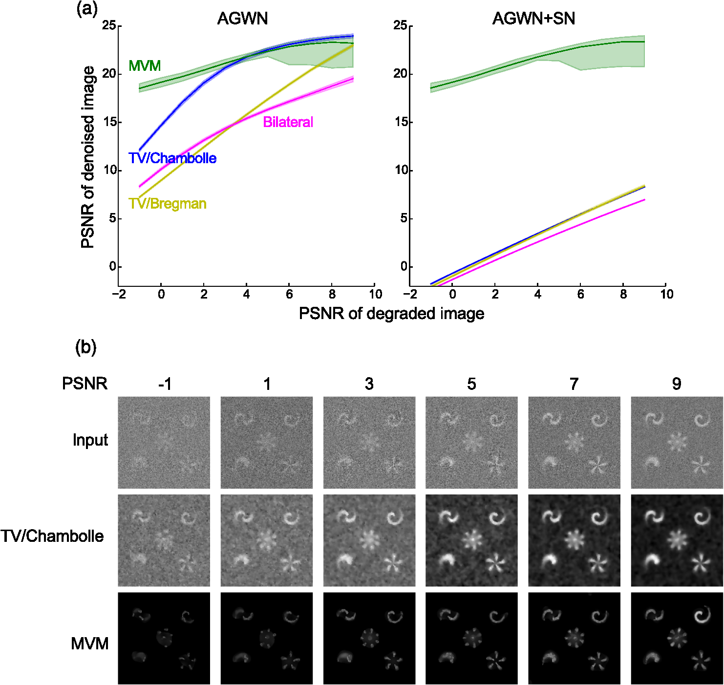 An important feature of the MVM is the ability to detect and segment structures in an input images, which is built in. Figure 6(a) presents the results of denoising of the test noisy phantom with TV/Chambolle, TV/Bregman, and the sure-let wavelet-based algorithm.25 SURE-LET denoising was done using the MATLAB® code provided by Luisier and colleagues.26 To detect individual objects in the output of the alternative denoising algorithms, we performed Otsu thresholding27 and labeled the resulting contiguous areas as individual objects. Because the given denoising techniques did not effectively suppress the salt noise present in the input phantom, we had to perform adaptive median filtering on the denoised images prior to Otsu segmentation. The results are presented in Fig. 6(b), where each object is shown in a different color. The object separation in MVM matches the ground truth of the object composition, while the alternative methods tend to segment some of the patterns into multiple objects. Some false-positive objects are also detected. It is likely that it is possible to tune the thresholding and segmentation algorithms for the other denoising methods to produce more satisfactory results, but in our view, the power of MVM is that this object separation comes out of the box. The TV/Chambolle produced the best results among the alternative denoising approaches and it was chosen for further comparison of the algorithm performance. Fig. 6Comparison of performance of MVM and other denoising techniques on the test noisy phantom, shown in Fig. 1(a). Denoising results for two total variation (TV) minimization techniqes with Chambolle and Bregman algorthms, bilateral filter and SURE-LET wavelet-based algorithm (a) and object segmentation and labeling results for the corresponding algorithms (b), segmentation is part of MVM, in other algorithms it was performed by labeling contiguous areas after binarization with automatic Otsu thresholding. 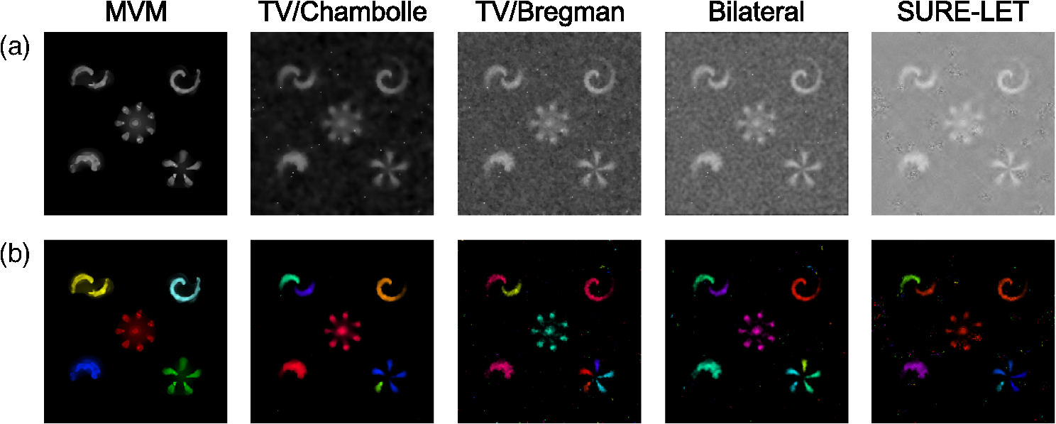 Figure 7 shows the results of the TV/Chambolle denoising and the MVM for the experimental data, displaying several glial waves co-occurring in the field of view (FOV). In short, we imaged spontaneous glial waves in mouse cerebellum in vivo under ketamine anesthesia using two-photon microscope and Oregon green BAPTA-1/AM dye. In the top row, every fourth frame of the original normalized frame sequence is shown (time interval between the shown frames is ). Fluorescence values in each pixel were normalized to their respective standard deviation after subtraction of the mean value. Experimental details are given in Refs. 15 and 18. Because we do not have ground truth for the events in the experimental data, we compared the denoising and detection results to operator-detected events. Locations of the five glial waves in the FOV as detected by the operator in the data are shown as circles in the fourth column of images. The TV/Chambolle denoising followed by Otsu thresholding and zeroing pixel values below the threshold (middle row) clearly improves the contrast of the images; however, there are also numerous above-threshold pixels which do not belong to any wave visible in the FOV. In contrast, the MVM (bottom row) provides a cleaner view of the data, recovering areas of elevated corresponding to glial waves, while at the same time rejecting background and providing for recognition of individual objects. Fig. 7Normalized fluorescence data (top row), results of TV/Chambolle denoising followed by Otsu thresholding and rejecting pixels below threshold (middle row), and results of the MVM reconstruction (bottom row). Objects, overlapping in neighboring frames are attributed to one signaling event and are shown in the same color code. Shown is every fourth frame of the original sequence, same data as in Fig. 4, there are several co-occurring calcium waves in the field of view (FOV). In the MVM. 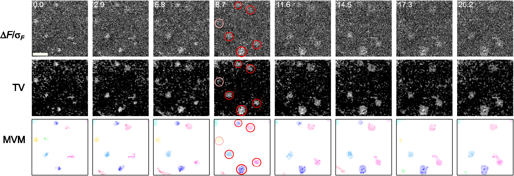 3.ConclusionOur aim in this work was to illustrate the utility of multiscale transforms for the extraction of useful signals from two-photon laser scanning microscopy imaging data. Our main point of application was detection and reconstruction of spontaneous glial waves using the multiscale vision model approach. In comparison to our previously reported MVM experience,18 we extended the technique by using the more robust mixed multiscale median/startlet transform for image decomposition and implemented an iterative scheme for nonlinear image restoration from the wavelet coefficients representing an object of interest. With this technique we were able to detect and reconstruct areas of increased elevations, corresponding to glial calcium waves and other forms of signaling in each of the recorded image frames. Performed in all frames, this procedure allows us to recover the whole dynamics of individual calcium waves by linking overlapping objects together in the neighboring frames. The mixed multiscale median/starlet transform allowed for suppression of both the Gaussian noise and outlying samples such as salt noise, while iterative object reconstruction from the significant wavelet coefficients and multiscale support allowed for a nearly perfect representation of the patterns, although the difference between the source image and the object reconstruction contained almost nothing but noise. With only minor modifications, MVM should be extendable to other applications, such as quantification of blood vessel cross-sectional areas, since penetrating vessels also appear as nearly circular structures in typical two-photon brain imaging data. There is obviously more to neuroimaging data than roundish calcium waves or vessel cross sections, and some native structures, such as Purkinje cell dendrites, are markedly anisotropic. Representation of such structures should benefit from using, for example, curvelet transforms.6 In general, it is probably a winning strategy to not limit the analysis to a single transform, but to combine the significant coefficients from several types of transforms, creating over-redundant dictionaries for morphological component analysis,2 which would allow for high flexibility in data representation. AcknowledgmentsWe thank Micael Lønstrup for providing excellent surgical assistance. This study was supported by the NORDEA Foundation/Center for Healthy Aging, the Lundbeck Foundation via the Lundbeck Foundation Center for Neurovascular Signaling (LUCENS), the NOVO-Nordisk Foundation, and the Danish Medical Research Council. ReferencesF. LuisierT. BluM. Unser,
“Image denoising in mixed Poisson-Gaussian noise,”
IEEE Trans. Image Process., 20
(3), 696
–708
(2011). http://dx.doi.org/10.1109/TIP.2010.2073477 IIPRE4 1057-7149 Google Scholar
J.-L. StarckF. MurtaghM.-J. Fadili, Sparse Image and Signal Processing: Wavelets, Curvelets, Morphological Diversity, Cambridge University Press, Cambridge, GB
(2010). Google Scholar
A Wavelet Tour of Signal Processing, Third Edition: The Sparse Way, 3rd ed.Academic Press, Burlington, MA
(2008). Google Scholar
B. Bathellieret al.,
“Wavelet-based multi-resolution statistics for optical imaging signals: application to automated detection of odour activated glomeruli in the mouse olfactory bulb,”
Neuroimage, 34
(3), 1020
–1035
(2007). http://dx.doi.org/10.1016/j.neuroimage.2006.10.038 NEIMEF 1053-8119 Google Scholar
J.-L. StarckM. EladD. Donoho,
“Redundant multiscale transforms and their application for morphological component separation,”
Adv. Imaging Electron Phys., 132 287
–348
(2004). http://dx.doi.org/10.1016/S1076-5670(04)32006-9 Google Scholar
J.-L. StarckE. J. CandèsD. L. Donoho,
“The curvelet transform for image denoising,”
IEEE Trans. Image Process., 11
(6), 670
–684
(2002). http://dx.doi.org/10.1109/TIP.2002.1014998 IIPRE4 1057-7149 Google Scholar
F. V. Wegneret al.,
“Fast XYT imaging of elementary calcium release events in muscle with multifocal multiphoton microscopy and wavelet denoising and detection,”
IEEE Trans. Med. Imaging, 26
(7), 925
–934
(2007). http://dx.doi.org/10.1109/TMI.2007.895471 ITMID4 0278-0062 Google Scholar
T. BluF. Luisier,
“The sure-let approach to image denoising,”
IEEE Trans. Image Process., 16
(11), 2778
–2786
(2007). http://dx.doi.org/10.1109/TIP.2007.906002 IIPRE4 1057-7149 Google Scholar
E. ScemesC. Giaume,
“Astrocyte calcium waves: what they are and what they do,”
Glia, 54
(7), 716
–725
(2006). http://dx.doi.org/10.1002/(ISSN)1098-1136 GLIAEJ 1098-1136 Google Scholar
T. M. Hooglandet al.,
“Radially expanding transglial calcium waves in the intact cerebellum,”
Proc. Natl. Acad. Sci. U S A, 106
(9), 3496
–3501
(2009). http://dx.doi.org/10.1073/pnas.0809269106 PNASA6 0027-8424 Google Scholar
J. W. DaniA. ChernjavskyS. J. Smith,
“Neuronal activity triggers calcium waves in hippocampal astrocyte networks,”
Neuron, 8
(3), 429
–440
(1992). http://dx.doi.org/10.1016/0896-6273(92)90271-E NERNET 0896-6273 Google Scholar
J. HungM. A. Colicos,
“Astrocytic Ca2+ waves guide CNS growth cones to remote regions of neuronal activity,”
PLoS One, 3
(11), e3692
(2008). http://dx.doi.org/10.1371/journal.pone.0003692 1932-6203 Google Scholar
K. Kanemaruet al.,
“Regulation of neurite growth by spontaneous Ca2+ oscillations in astrocytes,”
J. Neurosci., 27
(33), 8957
–8966
(2007). http://dx.doi.org/10.1523/JNEUROSCI.2276-07.2007 JNRSDS 0270-6474 Google Scholar
T. A. Weissmanet al.,
“Calcium waves propagate through radial glial cells and modulate proliferation in the developing neocortex,”
Neuron, 43
(5), 647
–661
(2004). http://dx.doi.org/10.1016/j.neuron.2004.08.015 NERNET 0896-6273 Google Scholar
C. Mathiesenet al.,
“Spontaneous calcium waves in Bergman glia increase with age and hypoxia and may reduce tissue oxygen,”
J. Cereb. Blood Flow Metab., 33
(2), 161
–169
(2013). http://dx.doi.org/10.1038/jcbfm.2012.175 JCBMDN 0271-678X Google Scholar
E. A. MukamelA. NimmerjahnM. J. Schnitzer,
“Automated analysis of cellular signals from large-scale calcium imaging data,”
Neuron, 63
(6), 747
–760
(2009). http://dx.doi.org/10.1016/j.neuron.2009.08.009 NERNET 0896-6273 Google Scholar
F. RueA. Bijaoui,
“A multiscale vision model to analyse field astronomical images,”
Exp. Astron., 7
(3), 129
–160
(1997). http://dx.doi.org/10.1023/A:1007984321129 EXASER 0922-6435 Google Scholar
A. BrazheC. MathiesenM. Lauritzen,
“Multiscale vision model highlights spontaneous glial calcium waves recorded by 2-photon imaging in brain tissue,”
Neuroimage, 68 192
–202
(2013). http://dx.doi.org/10.1016/j.neuroimage.2012.11.024 NEIMEF 1053-8119 Google Scholar
A. BijaouiF. Rué,
“A multiscale vision model adapted to the astronomical images,”
Signal Process., 46
(3), 345
–362
(1995). http://dx.doi.org/10.1016/0165-1684(95)00093-4 SPRODR 0165-1684 Google Scholar
J.-L. StarckF. Murtagh, Astronomical Image and Data Analysis, Springer, Berlin Heidelberg New York
(2006). Google Scholar
C. TomasiR. Manduchi,
“Bilateral filtering for gray and color images,”
in Proc. Int. Conf. Computer Vision,
839
–846
(1998). Google Scholar
A. Chambolle,
“An algorithm for total variation minimization and applications,”
J. Math. Imaging Vis., 20 89
–97
(2004). http://dx.doi.org/10.1023/B:JMIV.0000011320.81911.38 JIMVEC 0924-9907 Google Scholar
T. GoldsteinS. Osher,
“The split bregman method for l1-regularized problems,”
SIAM J. Img. Sci., 2
(2), 323
–343
(2009). http://dx.doi.org/10.1137/080725891 1936-4954 Google Scholar
S. van der Waltet al.,
“Scikit-image: image processing in python,”
PeerJ. PrePrints, 2 e453
(2014). http://dx.doi.org/10.7717/peerj.453 Google Scholar
F. LuisierT. Blu,
“Sure-let multichannel image denoising: interscale orthonormal wavelet thresholding,”
IEEE Trans. Image Process., 17
(4), 482
–92
(2008). http://dx.doi.org/10.1109/TIP.2008.919370 IIPRE4 1057-7149 Google Scholar
F. LuisierT. Blu,
“SURE-LET Wavelet Denoising,”
(2014) http://bigwww.epfl.ch/demo/suredenoising/ August ). 2014). Google Scholar
N. Otsu,
“A threshold selection method from gray-level histograms,”
IEEE Trans. Syst. Man Cybern., 9
(1), 62
–66
(1979). http://dx.doi.org/10.1109/TSMC.1979.4310076 ITSHFX 1083-4427 Google Scholar
BiographyAlexey Brazhe is a senior researcher in the Department of Biophysics, Biological faculty, Moscow State University. His research interests include mathematical modeling and multiscale signal and image analysis tools in application to neuroscience. He received his PhD degree in 2006 from Moscow State University. Claus Mathiesen is a postdoctoral fellow at Translational Neurobiology, University of Copenhagen. He received his PhD degree in 1990 from the University of Copenhagen and studies blood-brain-barrier mechanism, vascular and metabolic coupling to astrocytes, and neuronal activity in the aging brain. Barbara Lykke Lind is a postdoctoral fellow in the Department of Neuroscience and Pharmacology at the University of Copenhagen, Denmark. She is working in Martin Lauritzen’s group studying intracellular Ca2+ activities in astrocytes and neurons and the implications for the neurovascular coupling. She completed her PhD degree in 2014 at the University of Copenhagen. Andrey Rubin has been the head of the Department of Biophysics, Biological faculty, Moscow State University since 1976, and chair of the National Committee for Biophysics, Russian Academy of Science. Martin Lauritzen is a professor of clinical neurophysiology and head of the Department of Clinical Neurophysiology at Glostrup Hospital, and professor of translational neurobiology at the Department of Neuroscience and Pharmacology at the University of Copenhagen, Denmark. His research interests focus on the mechanisms coupling neuroglial activity to cerebral blood flow and energy metabolism, the underlying mechanisms for brain imaging, cortical spreading depression, and mechanisms of aging. |