2.1.

Instrumentation

To enable comparisons between usage of “short” and “very short” regressors (henceforth, S and VS, respectively), we modified an existing commercial high-density fiber probe (Cephalogics LLC, Boston, Massachusetts; for details see Ref. 10). As shown in Fig. 1, the basic geometry of 24 sources and 21 detectors was an interleaved rectangular grid with overall dimensions of $13.2\times 6.6\mathrm{cm}$. Nearest-neighbor diagonal distances were 13 mm, while the three next-nearest source-detector separations in the grid were 30, 39, and 47 mm.^6,10 The probe geometry was modified by moving three detectors (represented by dashed squares) to within 6 mm of sources in the grid. Three VS regression channels were thus created. For each, a single 13-mm channel sharing the same source was chosen as an S channel for comparison in the subsequent data analysis. Figure 1 indicates the locations of these pairs of channels, labeled as $A$, $B$, and $C$.

Fig. 1

Fiber bundle geometry for light delivery (circles) and detection (squares). In the unmodified regions of the rectangular grid, nearest-neighbor source-detector spacings are 13 mm (S channels), but relocated detectors are placed 6 mm from sources at labeled locations $A$, $B$, and $C$ to provide three VS channels. The circle around location $B$ (radius 25 mm) indicates the zone of target channels considered “near to $B$” in the data analysis; see text for details. N.B.: view from back (convex side) of the near-infrared spectroscopy headpiece. Key: dashed squares—vacated detector gridpoints, shaded squares—selected detectors for S/VS comparison.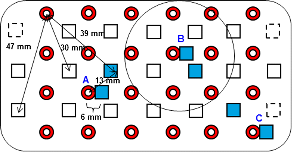

At each of the 24 source positions, optical fiber bundles delivered NIR light-emitting diode light at two wavelengths (750 and 850 nm). The bundles were coupled to the head with a flexible, thermoplastic cap molded to fit the back of the head over the visual cortex. Each detector sampled light from all sources for a total of 672 possible measurements; of these, the 265 channels with source-detector separations of 47 mm or less were retained for analysis. Further details about the system’s electronics have been published previously.¹⁰

Each time series of detected power at the two wavelengths was converted to changes in optical density and subsequently to changes in oxy- and deoxy-hemoglobin concentration times pathlength¹⁶ using the modified Beer-Lambert law. To render the changes in familiar units of average micromolar over the optically explored volume, the values were divided by a differential pathlength factor (DPF) of 5. This particular DPF, close to values reported for adults by Duncan et al.,¹⁷ does not affect any of the conclusions presented below and does not attempt to assign partial pathlength in the brain. Time series were high-pass filtered by subtracting a 25-s moving boxcar average and were low-pass filtered by performing a first-order Savitzky-Golay smooth¹⁸ over a 4-s window.

2.2.

Protocol

Visual stimulation was provided by a flickering black-and-white radial checkerboard pattern. The pattern was presented covering a 15-in. laptop screen, approximately 18 to 24 in. from the seated subject. During stimulus periods, the contrast of the pattern would reverse at a rate of 10 Hz. During rest periods, the subject was shown a solid gray screen with a small cross-hair in the center to maintain a central fixation point. The duration of the stimulations was 10 s, while the rest period was varied between 15 and 35 s to reduce habituation. A typical trial contained six visual stimulation epochs and lasted approximately 3 min.

Nine healthy subjects (age range: 19 to 40; four female) participated in this study, which was approved by the University of Rochester Research Subjects Review Board. Because most subjects sat for two trials, the total number of data runs was 17. The probe was placed over the occipital lobe, using the inion as a fiducial marker on the scalp. The center of the probe was placed approximately 1 to 2 cm above the inion, aligned along the midline. The probe’s width of 13.2 cm was enough to span the right and left occipital cortex.

3.1.

Correction Modalities

Every target channel’s time series of oxyhemoglobin concentration change was processed six separate times, once using each of the correction channels (3 VS and 3 S). The regression process, which has been described previously,⁸ performs scaled subtraction of the VS or S channel by least-squares minimization, producing a corrected time series. Each of the six regressions yielded a separate result. As a baseline for comparison, the data were also analyzed using no regressor at all.

Gagnon et al.⁴ have reported that correction channels provide more benefit if they are located within approximately 20 mm of the target channel, center-to-center. Since the headpiece in this study provided a range of center-to-center separations up to 40 mm, a wide range in correction quality was expected. For this reason, regressions were analyzed only for cases where the target channel’s midpoint was within 25 mm of the VS regressor’s midpoint (this radial distance from position $B$ is indicated by the large circle in Fig. 1). Since the VS and S midpoints were not identical, the center-to-center separations from each target channel were also different. In regions $A$ and $B$, there was no overall bias; in region $C$, the VS midpoint was always several millimeters farther away due to its placement at the edge of the probe. This created a bias against VS by reducing the spatial overlap, but since there were fewer channels corrected by $C$, the influence of this bias in the overall statistics was minor.

All target channels in our probe were within 25 mm of at least one 6 mm correction location ($A$, $B$, or $C$); some were that close to two.

3.2.

Metrics

Noise-reduction methods are most relevant in cases where there is an underlying signal to detect. This study focused upon channels in which stimulus-evoked activation signals were observed. To compare the noise-reduction methods quantitatively, a performance metric had to be developed. We quantified performance based upon the CNR of the activation responses, as will be described shortly.

By sensing extracerebral hemodynamics, short-distance correction methods reduce their contribution in target-channel measurements, ideally leaving “brain-only” responses behind. When stimulus-evoked hemodynamic activity has occurred in the brain (i.e., in the case of a “true positive”), the correction process should increase the CNR of the NIRS measurement. Our chosen performance metric therefore implies that higher CNR correlates with better correction.

It must be noted, however, that stimulus-evoked activity can instead occur in the extracerebral vasculature, for example, via a flushing response. Since the evoked hemodynamic signature appears in the short-distance measurement as well, the correction process will tend to reduce it in the target channel recording. In such instances (the correction of a “false positive”), the hallmark of proper correction is now a decrease in CNR. In a study with roughly equal numbers of true and false positives, CNR would be a poor metric for successful signal correction. In order to use CNR as a metric in this study, it was necessary to create a situation where true positives greatly outweighed false positives. The validity and limitations of this assumption will be revisited after the results are reported.

3.2.2.

CNR calculation

For each channel that passed the $t$-test, the corrected and uncorrected NIRS-measured oxyhemoglobin responses were each modeled using a skewed-Gaussian hemodynamic response function, as described previously.⁹ A fit was performed for each stimulus epoch over a 25-s window, starting at the onset of the 10-s stimulus and ending 15 s after the conclusion of the stimulus. As shown in Fig. 2, “contrast” (C) is defined as the maximum amplitude of the skewed-Gaussian fit, and “noise” is defined as four times the standard deviation of the residual, thus giving barely visible signals a CNR of approximately unity. The average CNR of a channel’s epochs served as an additional criterion for flagging activations ($\langle \mathrm{CNR}\rangle >1$). Specifically, this guarded against multipeaked hemodynamic oscillations that happen to pass the $t$-test by being randomly higher at the end of most epochs, but do not resemble single-peaked responses. In practice, all channels passing the $t$-test in these experiments also met the CNR criterion.

Fig. 2

An example of calculating contrast and noise values for a single stimulus epoch. The solid blue trace indicates the $\mathrm{\Delta }{\mathrm{HbO}}_2$ time series after regression against a 6-mm (VS) channel. The skewed-Gaussian fit (dashed magenta) results in a noise residual (green) whose standard deviation is calculated.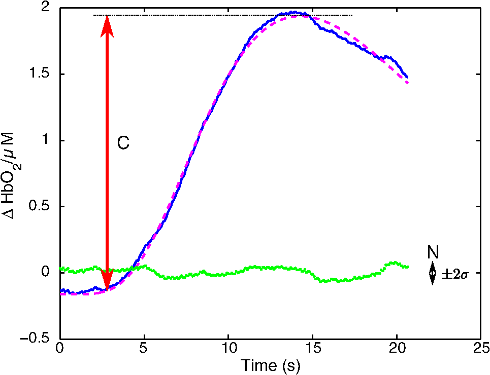

AFC status was assigned to a channel if the $t$-test and CNR criteria were both satisfied for at least one regression modality (S, VS, or NR).

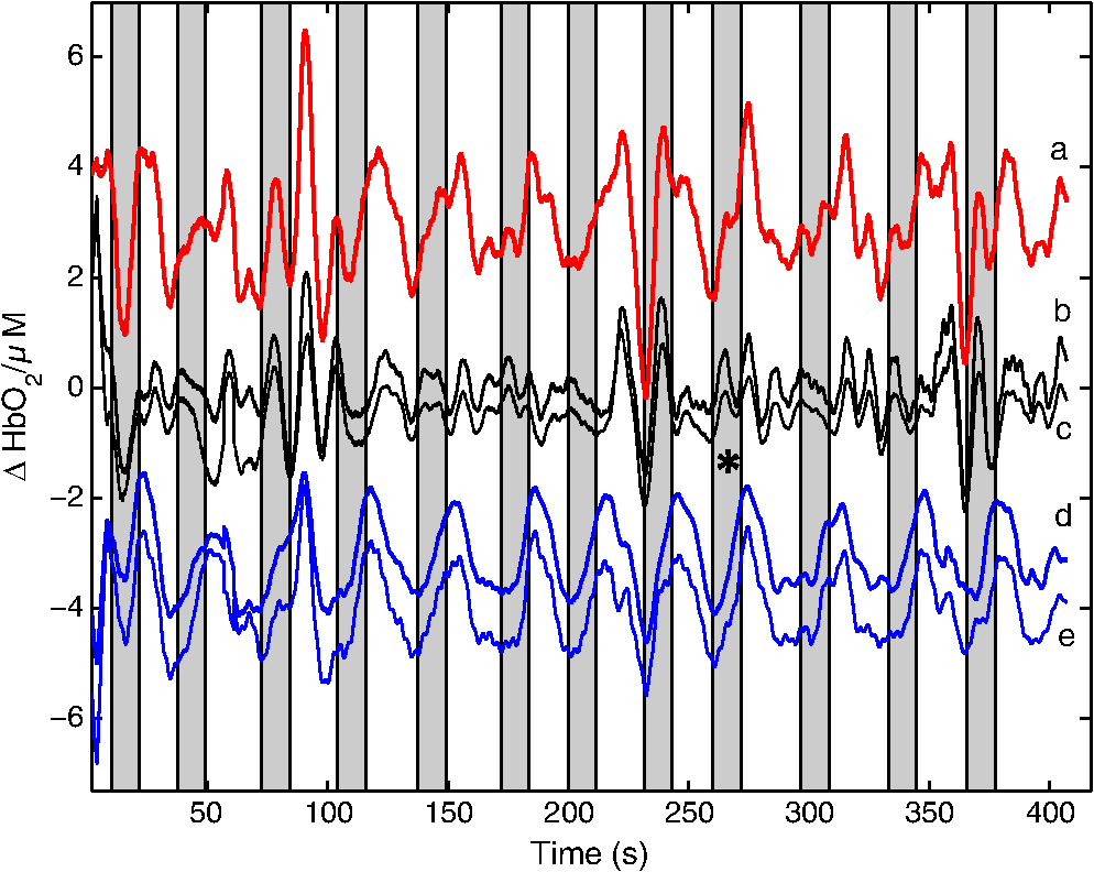4.1.

VS versus NR

Figure 4 compares very-short regression to NR. Specifically, ${\mathrm{CNR}}_{6\mathrm{mm}}$ was calculated for each AFC and scatter-plotted against the corresponding value of ${\mathrm{CNR}}_{\mathrm{NR}}$. As noted above, a few target channels were within 25 mm of two VS channels ($A$, $B$, or $C$); these channels have two data points in this figure, corresponding to correction by two different 6-mm channels. The scatter plot clearly shows most points (317 out of 467) lying above a 45-deg line, suggesting that the regression improved the CNR on average. The two-sided $t$-test of $\log ({\mathrm{CNR}}_{6\mathrm{mm}}/{\mathrm{CNR}}_{\mathrm{NR}})$ confirmed that the improvement was significant ($p<0.0001$). Significant improvement was also found for the S correction (data not shown). These results, consistent with prior work,⁹ serve as a baseline check before proceeding to comparisons of different correction methods.

Fig. 4

Scatter plot of contrast-to-noise ratio (CNR) from VS regression (6 mm) versus CNR from no-regression, for all “near-corrected” activation-flagged channels (AFCs) (correction channel 25 mm or closer to target channel, center-to-center). A dashed unity line is provided to guide the eye. 317 of the 467 data points have a higher CNR using VS regression, and the overall improvement is statistically significant ($p<0.0001$; see text for details).

This scatter plot also reveals information about the relative prevalence of true and false positives among the AFCs. Of the data points where the CNR in one modality is at least $2\times$ greater than the other, the larger CNR almost always belongs to the VS correction (i.e., such points lie above, not below, the unity line). According to the idealized model discussed earlier, if a correction method increases the CNR, this implies a true positive. Since almost all of the strong changes went in this direction, this suggests that the experimental design (adult volunteers watching a strong visual stimulus for many epochs) led to many more true positives than false positives.

4.2.

VS Versus S Regression

In Fig. 5, a scatter plot (similar to Fig. 4) compares ${\mathrm{CNR}}_{6\mathrm{mm}}$ to ${\mathrm{CNR}}_{13\mathrm{mm}}$, again for the cohort of all corrections within 25 mm. In this case, the number of data points above the 45-deg unity line is 326 out of 461. The smaller total number of data points, 461 compared to the 467 in Fig. 4, is due to six instances in which one of the S channels was itself flagged for activation; in these cases, S regression yielded an uninformative zero residual. The improvement was again statistically significant ($p<0.0001$).

Fig. 5

Scatter plots of CNR from VS regression (6 mm) versus CNR from S regression (13 mm), for all “near-corrected” AFCs. In 326 out of 461 instances, the VS regression has higher CNR, and the overall improvement in CNR is statistically significant ($p<0.0001$; see text for details).

4.3.

Global Regression

Since the global analysis could only be performed at 13 mm, there was no ability to compare global correction using VS and S modalities. Figure 6, however, illustrates an important relationship between the time course of a particular target channel (30 mm separation) and the global S average for that data run. As in Fig. 3, gray bars represent the stimulation epochs. The original 30-mm time series shows some amount of response correlated with the stimuli, but there is a lot of hemodynamic noise as well. In the corrected trace, plotted at the bottom, the hemodynamic interference is markedly reduced and the stimulus-related dynamics are noticeably smoother. No similar correction was observed in this case when a single nearby channel (either VS or S) was used as the regressor; the residual still contained most of the higher-frequency noise (data not shown).

Fig. 6

Oxyhemoglobin trends recorded using a single 30-mm channel (thick red upper trace) and the global average of the 13-mm channels (thin black upper trace, scaled for least-squares fit). Gray bars indicate stimulation epochs. The corrected time series (blue bottom trace) exhibits surges at the onset of each stimulation, with significant reduction in unrelated hemodynamic activity (e.g., around 95 s). In this instance, local correction provided no comparable reduction (data not shown).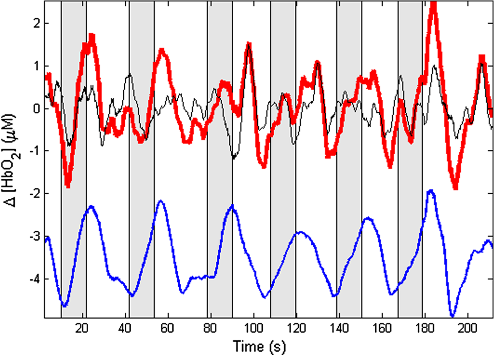

Fig. 7

Oxyhemoglobin trends recorded using a 13-mm channel (a, red) and the corresponding 6-mm channel sharing the same source (b, black, scaled for least-squares fit). Gray bars indicate stimulation epochs. The residual of the fit (c, blue, magnified for clarity by a factor of 5) exhibits surges at the onset of each stimulation, suggesting that the 13-mm recording has significant sensitivity to stimulus-related hemodynamics.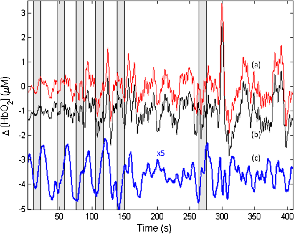

In the example shown, the average CNR of the activations in the global regression was six times greater than the local regression (36 versus 6). Although this was an extreme example shown here for emphasis, the effect was not isolated. Averaging over all of the AFCs in this study, global-average S regression produced higher CNR values for 271 of the flagged channels, versus 196 being better with single-channel VS regression.

5.1.

VS Versus S Regression

As mentioned in Sec. 1, the major goal of this investigation was to compare two relevant source-detector separations for short-distance regressor channels. For this reason, the optical headpiece for this study was built with three pairs of regression channels at 6 and 13 mm, each pair sharing a common source. Time series from many target channels were then corrected using either 6-mm (VS) or 13-mm (S) channel data. Since the three relevant time series were acquired in parallel (target channel, VS regressor, and S regressor), all other variables were held fixed in the comparison of the regression results.

As Fig. 5 shows, overall the 6-mm VS regressor performed significantly better than the 13 mm S regressor, as measured by the CNR of the stimulus-related activations that were flagged. This suggests that 6 and 13 mm, although both regarded as distances too short to obtain an optimal sampling of the adult human cortex, are not functionally equivalent in terms of their hemodynamic probing.

One hypothesis for the difference in performance is that the 13-mm channel sensed some cortical hemodynamics itself. Using such a channel for regression would naturally subtract some of the signal one wishes to preserve. We have seen direct evidence of 13-mm channels containing significant activation signals in some of our data. For example, the upper trace in Fig. 7 shows a 13-mm NIRS time course collected from one of the subjects. No obvious stimulus-related features are apparent. When this channel is regressed against its associated 6-mm channel, however, the residual exhibits upward surges in oxyhemoglobin concentration at the onset of each stimulus block. In this instance, the 13-mm channel evidently contained significantly higher levels of cerebral activation signal than the 6-mm channel did. This would agree with the results in Fig. 5, where the CNR was statistically worse using 13-mm regression.

5.2.

Global Regression

The global average at 13 mm sometimes provided a strong correction to a far-distance channel (cf. Fig. 6), and overall produced higher CNR than single-channel correction in a majority of cases. These findings emphasize that there are multiple potential sources of hemodynamic interference, and that no one correction approach is always the best choice. In the case where superficial hemodynamics are the dominant interferent, a local superficial channel ought to be the best regressor. In the case shown in Fig. 6, however, the dominant interference was better explained by a global average over a larger area. The “global interferent” in this case could have been predominantly in the brain, and thus poorly sampled by the VS channels.

This study leaves open the question of whether global regression is improved by switching to 6-mm channels, as was seen for single-channel regression. Such a comparison would require a probe with a full complement of 6-mm regression channels, which was not available in this study.